What to practice
- distinguish variables, controls, replicates and statistical claims
Read every investigation in five steps
Use the same five questions whenever a prompt describes an experiment, a table or a graph.
- Question. What relationship is being tested?
- Comparison. What was changed, and which entities independently received each treatment?
- Measurement. What was measured, in what units, and when?
- Result. What pattern appears, and how uncertain is it?
- Inference and limit. What claim do the data support, and what can this design not establish?
A result reports a pattern ("treated plants were taller"). An inference explains or generalizes it ("fertilizer increased growth under these conditions"). A limit names what the design cannot show ("one variety was grown for 21 days"). Keep them separate. Every experimental scenario and data set in this chapter is hypothetical data for practice.
Variables and the comparison that answers the question
The independent variable is the condition the investigator deliberately changes. The dependent variable is the measured response, always with units. Controlled variables are kept the same so that they cannot explain a difference. A control is a comparison chosen to answer a specific question.
Worked demonstration: name what each control rules out
A student asks whether a leaf extract slows the growth of a bacterium. Paper disks soaked in extract at 0, 25, 50 and 100 percent strength go on separate agar plates spread with the bacterium. After 24 hours at 30 °C, the student measures the clear zone around each disk.
Extract strength is the independent variable; clear-zone diameter (mm) is the dependent variable. Agar volume, bacterial density, disk size, liquid per disk, temperature and time are controlled.
The extract was made in dilute ethanol, so the 0 percent disk, soaked in that solvent alone, is the negative control. It asks: does the solvent by itself produce a clear zone? A disk carrying an antibiotic known to inhibit this bacterium is the positive control. It asks: can this assay detect inhibition at all? If the antibiotic disk shows no clear zone, extract disks without clear zones say nothing about the extract.
"Add a control" earns little, because it does not say which explanation the control removes. Name the comparison and its purpose.
Try it 3.1. A student germinates 20 bean seeds in light on a warm windowsill and 20 in a dark cupboard in a cool room. Identify the independent and dependent variables, explain why the design cannot isolate the effect of light, and propose a repair.
Replicates, experimental units and sample size
The experimental unit is the entity that independently receives a treatment. Sample size, n, counts experimental units per group. Repeated readings of one unit improve that unit's measurement; they do not create new units (NC3Rs definition of the experimental unit). Miscounting units inflates n and makes weak evidence look strong, a problem documented in published laboratory research (Lazic and colleagues, PLOS Biology, 2018).
Worked demonstration: count pots, not readings
Twelve pots each hold one radish plant. Six are randomly assigned fertilizer and six receive none; all stand on one bench. After 21 days, each plant's height is read three times. Fertilizer was assigned pot by pot, so the pot is the experimental unit. Average the three readings into one value per pot: n = 6 per group, not 18. Random assignment spreads unmeasured differences, such as seed vigor, across both groups, but chance variation remains and must still be estimated.
Try it 3.2. Another student puts 9 plants in one fertilized tray and 9 in one unfertilized tray, then reports n = 9 per group. Identify the experimental unit and the actual n, and redesign the study with the same 18 plants.
Describe data: mean, standard deviation and standard error
These are the relationships given on the official reference sheet:
The standard deviation, s, describes how much individual values vary. The standard error of the mean describes how precisely the sample mean estimates the mean of all similar units. Because n sits under a square root, larger samples shrink SE; they do not systematically shrink SD.
Worked demonstration: summarize the unfertilized pots
The six unfertilized pot means are 8.2, 9.1, 7.6, 8.8, 9.4 and 8.3 cm. Their mean is 51.4 ÷ 6 = 8.57 cm.
| Pot mean (cm) | 8.2 | 9.1 | 7.6 | 8.8 | 9.4 | 8.3 |
|---|---|---|---|---|---|---|
| Deviation | −0.37 | 0.53 | −0.97 | 0.23 | 0.83 | −0.27 |
| Squared | 0.134 | 0.284 | 0.934 | 0.054 | 0.694 | 0.071 |
The squared deviations sum to about 2.17. Divide by n − 1 = 5 to get 0.434; the square root gives s ≈ 0.66 cm. Then SE = 0.659 ÷ √6 ≈ 0.27 cm. Keep unrounded values until the end. The fertilized pots have a mean of 10.33 cm, s ≈ 0.66 cm and SE ≈ 0.27 cm.
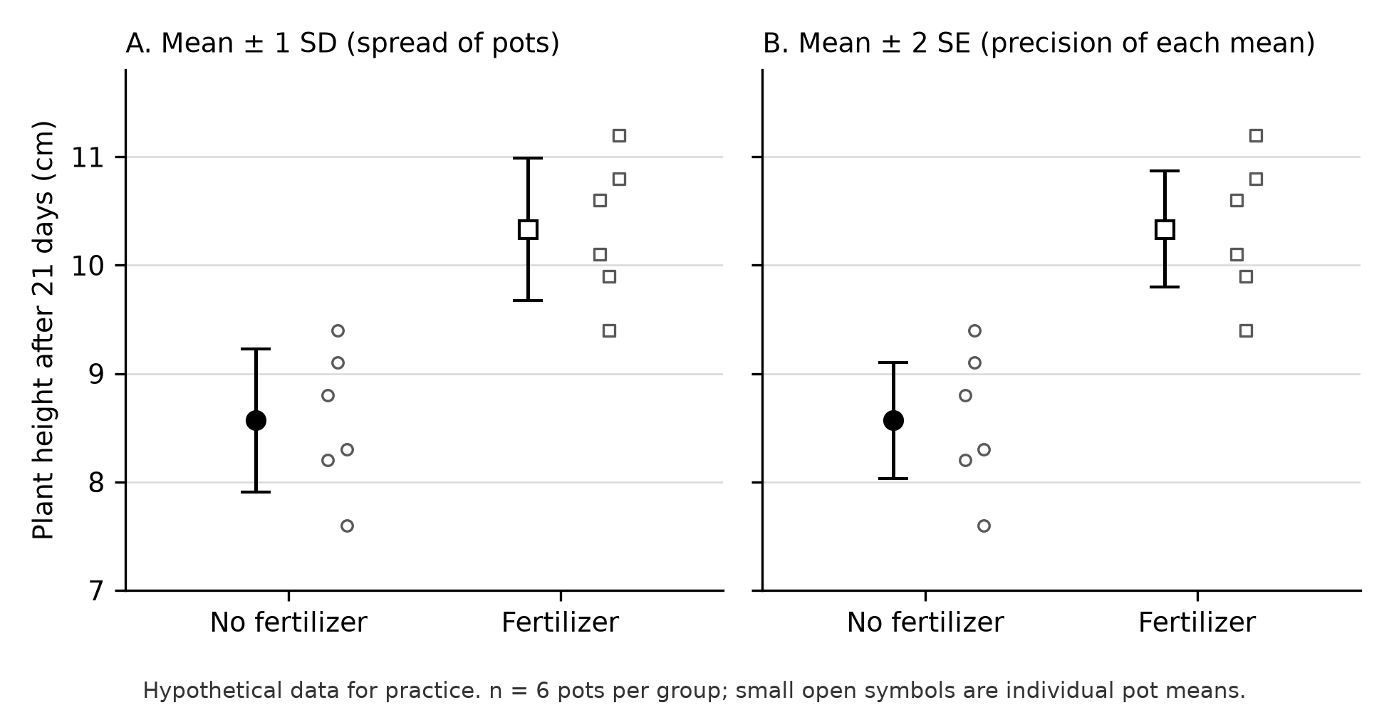
Figure 3.1. The same hypothetical pot data drawn two ways: ±1 SD bars show spread among pots (A); ±2 SE bars show the precision of each mean (B). Small open symbols are individual pots (n = 6 per group).
Read error bars before comparing them
Error bars may show SD, SE, a multiple of SE or a confidence interval, and each says something different; unlabeled bars cannot support an inference (Cumming, Fidler and Vaux, Journal of Cell Biology, 2007).
- Find the label first. SD bars describe spread, so their overlap does not test whether means differ.
- Know what ±2 SE approximates. With about ten or more units per group, ±2 SE is close to a 95 percent confidence interval for the mean; with very small samples the 95 percent interval is wider than ±2 SE (NIST explanation of confidence intervals).
- Read overlap in one direction. When ±2 SE bars or 95 percent intervals for two independent groups do not overlap, the data give good evidence that the means differ. Overlap leaves the difference uncertain; it does not prove the means are equal. If a prompt states a convention, apply it and qualify your claim.
- Compare independent groups. Bars on repeated measurements of one group cannot judge that group's change over time.
In Figure 3.1B the intervals, about 8.0–9.1 cm and 9.8–10.9 cm, do not overlap. The data support the claim that fertilizer increased mean height for this variety on this bench over 21 days. They do not show which nutrient was responsible or how it acted.
Try it 3.3. Use Figure 3.1. (a) Which panel answers, "How much did individual pots differ?" (b) Why would unlabeled bars prevent the Panel B conclusion?
Try it 3.4. Four independently grown cultures produce 12, 15, 9 and 12 units of a pigment. With a four-function calculator that has a square-root key, find the mean, s and SE.
Choose a graph that matches the variables
Put the independent variable on the x-axis and the dependent variable on the y-axis, each labeled with units. For categories, such as treatments or species, use a bar graph or dot plot of means with labeled error bars, and never connect categories with lines. For a continuous variable, such as time or concentration, use a scatterplot; connect points or add a best-fit line only when the trend is the claim. Start bar graphs at zero. Chapter 22 practices full graph construction.
Test a genetic model with chi-square
A chi-square goodness-of-fit test asks whether observed counts differ from a model's expected counts by more than chance usually produces (NIST description of the chi-square goodness-of-fit test).
The null hypothesis states that the model explains the data and deviations reflect chance. Degrees of freedom equal the number of categories minus one. The reference sheet's critical values at p = 0.05 are 3.84 for one degree of freedom, 5.99 for two and 7.81 for three. If χ² exceeds the critical value, reject the null hypothesis; otherwise, fail to reject it.
Worked demonstration: a 3 : 1 prediction
Two plants of a fictional species, both heterozygous for stem color, produce 141 purple and 59 green offspring. If purple is completely dominant and all offspring survive equally, a 3 : 1 model predicts 150 purple and 50 green among 200.
With two categories, df = 1. Because 2.16 < 3.84, fail to reject: the counts are consistent with a 3 : 1 model. That is not proof; another model might fit too. Use counts, never percentages, because χ² depends on sample size. Entering these results as 70.5 and 29.5 percent would give a wrong χ² of 1.08.
Try it 3.5. A cross between plants of this species heterozygous for two genes predicts 9 : 3 : 3 : 1. Among 160 offspring, the classes contain 72, 44, 30 and 14 plants, in the model's order. Calculate χ², decide at p = 0.05, and explain what the decision does and does not tell you.
Set up a Hardy–Weinberg problem
For one gene with two alleles, p and q are the two allele frequencies:
Separate two questions. What are the allele frequencies? When genotype counts are known, count allele copies directly; no equilibrium assumption is needed. What genotype frequencies would equilibrium predict? Only then use p², 2pq and q², which assume no mutation, random mating, no migration, no selection and a very large population. Real populations rarely meet all five, so the model is a baseline for comparison (OpenStax Biology 2e, Population Evolution).
Worked demonstration: count first, predict second
A beetle population has 260 AA, 180 Aa and 60 aa individuals: 500 beetles carrying 1,000 allele copies.
So q = 0.30. Equilibrium predicts 0.49 × 500 = 245 AA, 0.42 × 500 = 210 Aa and 0.09 × 500 = 45 aa. There are fewer heterozygotes than predicted; Chapter 18 tests such gaps.
Beware the shortcut. √(60/500) gives q ≈ 0.35, not 0.30, because treating the aa frequency as q² assumes equilibrium. Use it only when equilibrium is stated and genotype counts are unavailable.
Try it 3.6. In a flower population of 1,600 plants assumed to be in Hardy–Weinberg equilibrium, 256 show the recessive white phenotype. Find q, p and the expected number of heterozygotes. Explain why these data cannot test the equilibrium assumption.
Rates, ratios and percent change
A rate divides the change in a measured quantity by the time it took:
State units and the interval. On a cumulative graph the rate is the slope; if the curve bends, use the early, nearly straight portion and name it.
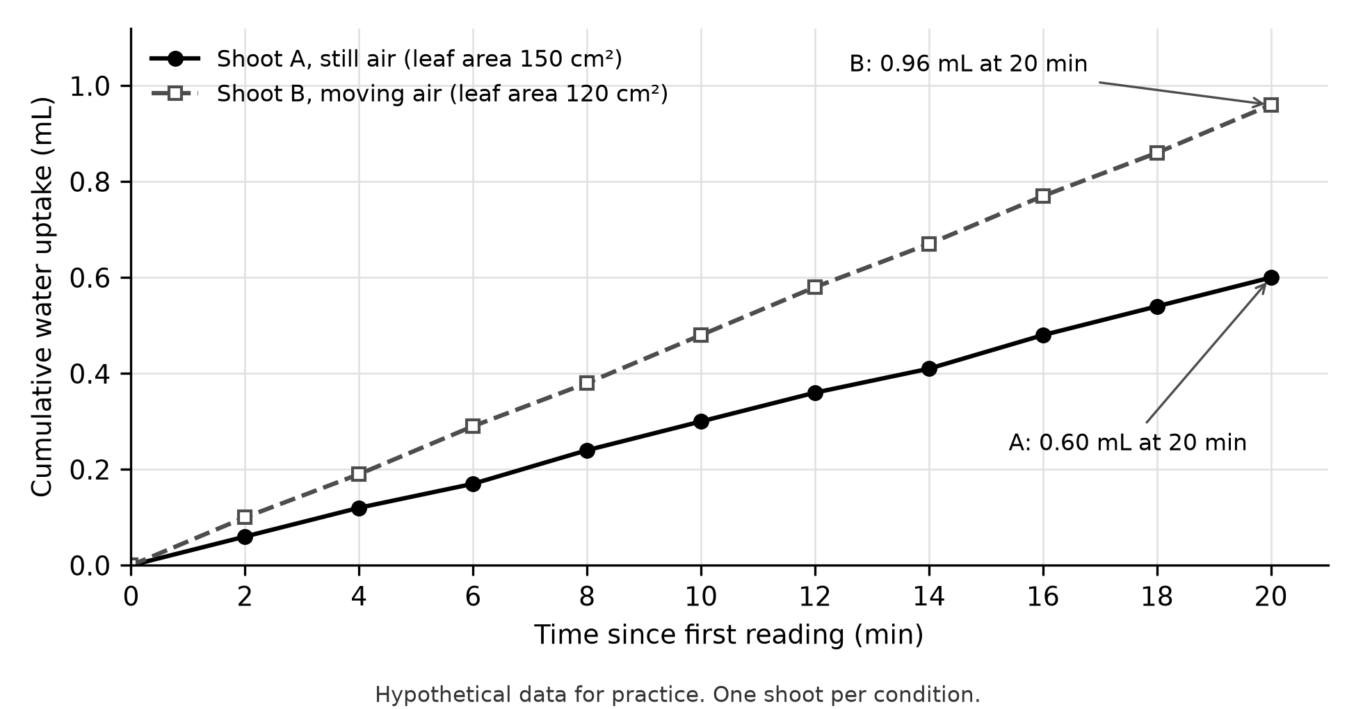
Figure 3.2. Hypothetical potometer readings for one leafy shoot in still air (leaf area 150 cm²) and one in fan-moved air (leaf area 120 cm²).
Worked demonstration: normalize before comparing
Both lines are nearly straight, so use 0–20 minutes. Shoot A: 0.60 mL ÷ 20 min = 0.030 mL/min, or 30 µL/min. Shoot B: 0.96 mL ÷ 20 min = 48 µL/min. In raw rates, B is (48 − 30) ÷ 30 × 100 = 60 percent higher.
Most water leaves a shoot through its leaves, so leaf area alone can change uptake. Per cm² of leaf, A takes up 30 ÷ 150 = 0.20 µL/min and B takes up 48 ÷ 120 = 0.40 µL/min: 100 percent higher. Normalizing changed the size of the comparison. The limit is severe: with one shoot per condition, air movement cannot be separated from other differences between the shoots.
Percent change differs from percentage-point change. Germination rising from 40 to 50 percent is a 10-percentage-point increase but a 25 percent relative increase.
Try it 3.7. A third still-air shoot with 200 cm² of leaves takes up 0.84 mL in 20 minutes. (a) Find its rate in µL/min and per cm². (b) Compare it with Shoot A.
Surface area and volume
Materials cross a cell's surface, while demand for them depends on its volume. As a cell grows, surface area rises with the square of its length but volume rises with the cube, so the surface area-to-volume ratio falls (OpenStax Biology 2e, cell size).
Worked demonstration: double the radius
For a sphere, SA = 4πr² and V = (4/3)πr³, so SA/V = 3/r. A cell of radius 5 µm has SA ≈ 314 µm², V ≈ 524 µm³ and a ratio of 0.6 per µm. At 10 µm, area quadruples and volume rises eightfold, so the ratio halves to 0.3 per µm: each unit of cytoplasm has half as much membrane serving it.
Try it 3.8. Two cells each have a volume of 100 µm³: a flat 10 × 10 × 1 µm slab and a 5 × 5 × 4 µm box. Using SA = 2lw + 2lh + 2wh, compare their ratios and explain which exchanges materials more readily.
Predict water movement with water potential
Water potential, Ψ, compares the potential energy of water with that of pure water and predicts which way water moves. Water moves from higher to lower water potential; pure water at atmospheric pressure is defined as zero (OpenStax Biology 2e, water potential).
Here i is the number of particles per solute unit (1 for sucrose), C is molar concentration, R = 0.0831 L·bar/(mol·K) and T is in kelvins (°C + 273). Solutes make negative; in an open container, = 0.
Worked demonstration: plant tissue in sucrose
A 0.30 mol/L sucrose solution stands in an open beaker at 22 °C (295 K). With i = 1, the units cancel to bar:
With = 0, the solution's Ψ is −7.35 bar. (An idealized 0.15 mol/L NaCl solution, with i = 2, gives the same value.) Cells in a piece of plant tissue have = −8.0 bar and = +2.0 bar, so their Ψ is −6.0 bar. If water crosses the membranes but sucrose does not, water moves from −6.0 toward −7.35 bar, out of the cells, and the tissue loses mass. The cells hold more solute than the solution, yet water leaves; pressure potential changed the prediction.
Common errors: dropping the negative sign, using degrees Celsius, setting a salt's i to 1, and comparing only solute potentials when pressure potentials differ.
Try it 3.9. Plant cells with = −6.0 bar and = +0.5 bar are placed in 0.20 mol/L sucrose in an open beaker at 27 °C. Calculate the solution's water potential, predict net water movement, and describe how changes as water moves.
Plan dilutions
The dilution relationship C₁V₁ = C₂V₂ is not on the official reference sheet, but laboratory descriptions rely on it. C₁ and V₁ describe the stock and the volume taken; C₂ and V₂ describe the concentration and total volume wanted.
Worked demonstration: make a working solution
For 50 mL of 0.20 mol/L sucrose from a 1.0 mol/L stock, V₁ = (0.20 × 50 mL) ÷ 1.0 = 10 mL. Measure 10 mL of stock and add water to a total of 50 mL, about 40 mL of water. Adding 50 mL of water would make 60 mL of a weaker solution. In a serial dilution, each step applies the same factor: three 1-in-10 steps dilute the original 1 in 1,000.
Try it 3.10. (a) How would you make 25 mL of 0.40 mol/L sucrose from a 2.0 mol/L stock? (b) A bacterial culture is diluted 1 in 10 four times. Spreading 0.10 mL of the final dilution yields 47 colonies. Assuming each colony grew from one viable cell, estimate viable cells per mL in the original culture.
Formula guide for study
This study aid is not the official AP Biology reference information.
| Task | Relationship | Check |
|---|---|---|
| Spread or precision | s; SE = s/√n | Is n the number of independent units? |
| Fit to a model | χ² = Σ(o − e)²/e | Counts, not percentages; df = categories − 1 |
| Allele frequency | p + q = 1 | Count allele copies when genotypes are known |
| Equilibrium prediction | p² + 2pq + q² = 1 | Is equilibrium stated? |
| Rate | ΔY/Δt | Units, interval, normalization |
| Cell size | SA/V | Squared versus cubed units |
| Water movement | ; | Negative sign, kelvins, i |
| Dilution | C₁V₁ = C₂V₂ | V₂ is the final total volume |
Check your try-it work
3.1. Light is the independent variable; germination percentage is the dependent variable. Temperature also differs, so it could cause any difference. Repair: keep all seeds in one location at one temperature and randomly assign containers either to light or to opaque covers.
3.2. Fertilizer was applied to whole trays, so the tray is the experimental unit and n = 1 per group; any tray difference is confounded with treatment. Better: pot the 18 plants separately and randomly assign 9 pots to each treatment, with positions mixed.
3.3. (a) Panel A, because SD describes spread among pots. (b) Without labels, the reader cannot tell spread from precision, so overlap or separation has no defined meaning.
3.4. Mean = 48 ÷ 4 = 12. Deviations 0, 3, −3 and 0 give squared deviations summing to 18. s = √(18 ÷ 3) = √6 ≈ 2.45 units; SE = 2.45 ÷ √4 ≈ 1.22 units.
3.5. Expected counts: 90, 30, 30, 10. χ² = 324/90 + 196/30 + 0/30 + 16/10 = 3.60 + 6.53 + 0 + 1.60 = 11.73. With df = 3, 11.73 > 7.81, so reject the 9 : 3 : 3 : 1 model at p = 0.05. The counts are unlikely if the model's assumptions, such as independent assortment and equal survival, all hold. The test does not identify which assumption failed; linkage or unequal survival would need further evidence.
3.6. q² = 256 ÷ 1,600 = 0.16, so q = 0.4 and p = 0.6. Expected heterozygotes = 2(0.6)(0.4)(1,600) = 768. Dominant-phenotype plants include both AA and Aa, whose counts are unknown, and finding q already required assuming equilibrium, so the data cannot test it.
3.7. (a) 0.84 mL ÷ 20 min = 42 µL/min; 42 ÷ 200 ≈ 0.21 µL/min per cm². (b) Its raw rate is 40 percent above Shoot A's 30 µL/min, but per cm² the rates are nearly equal (0.21 versus 0.20). Leaf area accounts for most of the raw difference.
3.8. Slab: SA = 200 + 20 + 20 = 240 µm², ratio 2.4 per µm. Box: SA = 50 + 40 + 40 = 130 µm², ratio 1.3 per µm. The slab has more membrane per unit volume, so it exchanges materials more readily.
3.9. T = 300 K, so = −(1)(0.20)(0.0831)(300) ≈ −4.99 bar, which is also the solution's Ψ. The cells' Ψ = −6.0 + 0.5 = −5.5 bar, so water moves from the solution into the cells. As the wall resists expansion, rises until the water potentials are equal and net movement stops.
3.10. (a) V₁ = (0.40 × 25) ÷ 2.0 = 5.0 mL of stock, plus water to a total of 25 mL (about 20 mL). (b) The final tube is a 1 in 10,000 dilution. 47 ÷ 0.10 mL = 470 cells per mL there; multiplied by 10,000, the original holds about 4.7 × 10⁶ viable cells per mL.
Practice
This chapter has no numbered bank questions; its practice is Try it 3.1 to 3.10. Work each with a four-function or scientific calculator before reading Check your try-it work above, and log every error by type. In one week, redo 3.4, 3.5, 3.6 and 3.9 on blank paper. Later chapters apply these tools: surface area and water potential in Chapters 6–7, rates in 8–9, chi-square in 13, Hardy–Weinberg in 18, population data in 20–21 and complete graphing in 22.