What to practice
- calculate frequencies and identify the assumptions of a model
At the population scale, evolution is a change in allele frequencies across generations. Chapter 17 explained natural selection. This chapter adds mutation, genetic drift and gene flow, and a model, Hardy–Weinberg equilibrium, of a population in which none of the four acts. Data sets without a cited source are hypothetical.
Count alleles, not individuals
A population's gene pool is every copy of every allele its members carry. For one gene with two alleles, an allele frequency is the fraction of gene copies that are one allele. A genotype frequency is the fraction of individuals with one genotype. A diploid population of N individuals holds 2N copies of each autosomal gene, so allele frequencies use 2N as the denominator.
Worked example 18.1: allele frequencies from genotype counts
A biologist uses a DNA test to genotype 150 marsh mice at a marker gene with alleles M and m: 63 MM, 69 Mm and 18 mm. Each MM mouse carries two M copies and each Mm mouse carries one.
Check that p + q = 1. This calculation assumes nothing about equilibrium. Two errors are common: dividing by 150, which counts mice rather than gene copies, and reporting (63 + 69)/150 = 0.88, the fraction of mice that carry M.
Try it 18.1. A sample of 250 lizards contains 40 BB, 110 Bb and 100 bb. (a) Find the frequency of b. (b) What fraction of the lizards carry at least one b? Explain why the two answers differ.
Four processes that change allele frequencies
A change in allele frequencies over generations is evidence that a population is evolving, and four processes can cause one (AP Biology Course and Exam Description, topics 7.4–7.5; OpenStax Biology 2e, Population Genetics).
- Mutation creates new alleles. Mutations arise at random with respect to an organism's needs; a mutation is not more likely because it would help. At any one gene, new mutations are rare, so mutation alone shifts frequencies slowly, but it supplies the variation that the other processes act on.
- Genetic drift is change caused by chance in which individuals survive, mate and pass on which alleles. It is stronger in small populations, where each individual is a larger share of the gene pool. A bottleneck occurs when a population is reduced to a few individuals for at least one generation. A founder effect occurs when a few individuals start a new, separate population. Either way, the survivors' or founders' alleles are a chance sample: some alleles become more common and others disappear.
- Gene flow, or migration, adds or removes alleles as individuals or gametes move between populations. It makes populations more alike and can keep them from diverging into separate species.
- Natural selection changes allele frequencies when heritable differences cause some individuals to leave more offspring than others in a particular environment.
Only selection consistently increases alleles that improve reproduction in the current environment. Drift can fix a harmful allele or remove a helpful one, especially in small populations.
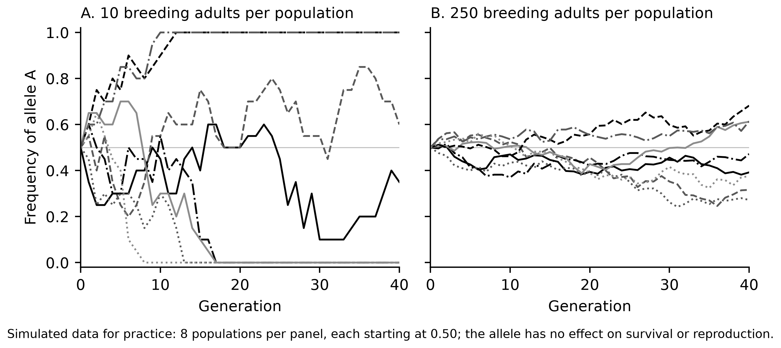
Figure 18.1. Simulated genetic drift of an allele that does not affect survival or reproduction. By generation 40, the allele was lost from four of the eight small populations and fixed in two. None of the large populations lost or fixed it.
Worked reasoning 18.2: drift or selection?
Ten beetle populations of 30 adults began with allele E at a frequency of 0.40. Five were kept in heated chambers and five at room temperature. After 15 generations, the frequency of E had changed as follows.
| Treatment | Change in frequency of E in each population | Mean change |
|---|---|---|
| Heated | +0.21, +0.18, +0.25, +0.16, +0.22 | +0.20 |
| Room temperature | +0.06, −0.09, +0.11, −0.04, −0.02 | +0.00 |
Drift is random in direction, so replicate populations scatter both ways, as the room-temperature group did. Five gains out of five in heat are unlikely from drift alone, which points to selection on E or a gene near it. Drift still acted there too, which is why the gains ranged from 0.16 to 0.25. A change in frequency shows only that a population evolved; replicates and a comparison group are what let you name the process.
Try it 18.2. Name the process in each case and state whether its direction is random. (a) A storm leaves 12 surviving birds on an island, and their descendants rebuild the population. (b) Five seeds carried by a bird start a new plant population on a lake island. (c) Pollen from a neighboring field reaches a wheat field every year. (d) A copying error during DNA replication produces a new allele in one sperm cell.
Hardy–Weinberg: a model of a population that is not evolving
The Hardy–Weinberg model describes allele and genotype frequencies that stay constant from one generation to the next (OpenStax Biology 2e, Population Evolution). For one gene with two alleles at frequencies p and q:
The terms p², 2pq and q² are the expected frequencies of the three genotypes. The model assumes gametes combine at random. An offspring receives allele A from each parent with probability p, so AA has probability p × p. A heterozygote can form two ways, A from the mother and a from the father or the reverse, which is why the middle term is doubled.
Five conditions keep the frequencies constant: a very large population (no drift), no migration, no new mutations, random mating and no natural selection. Real populations never meet all five. That is what makes the model useful as a null hypothesis: it predicts what you would observe if nothing were changing the gene pool, so a clear mismatch is evidence that at least one condition fails.
Consider nonrandom mating. When individuals mate mostly with similar individuals or relatives, or when plants self-pollinate, more offspring are homozygous. Heterozygotes become scarcer, but nonrandom mating by itself does not change allele frequencies.
Worked example 18.3: use q² only when equilibrium is stated
A large cattle herd is stated to be in Hardy–Weinberg equilibrium for a gene whose recessive allele causes a visible condition in 1 of every 400 calves. What fraction of calves are carriers?
q² = 1/400 = 0.0025, so q = √0.0025 = 0.05 and p = 0.95. Carriers = 2pq = 2(0.95)(0.05) = 0.095, about 1 calf in 10.5. Most copies of a rare recessive allele sit in heterozygotes, not in affected calves.
This shortcut works only because equilibrium was stated and the dominant phenotype hides two genotypes. When genotype counts are available, count alleles directly, as in Worked example 18.1.
Test a population against Hardy–Weinberg with chi-square
A biologist genotypes 200 plants of a self-compatible wildflower at a DNA marker gene and finds 81 AA, 78 Aa and 41 aa. Are these counts consistent with Hardy–Weinberg expectations?
Worked example 18.4: the complete test
Step 1. State the hypotheses. Null: the population is in Hardy–Weinberg equilibrium for this gene, and deviations reflect chance in sampling. Alternative: genotype frequencies differ from equilibrium expectations.
Step 2. Find the allele frequencies. p = (2 × 81 + 78)/400 = 240/400 = 0.60, so q = 0.40.
Step 3. Find the expected counts. Multiply each equilibrium frequency by 200: AA is 0.36 × 200 = 72, Aa is 0.48 × 200 = 96, and aa is 0.16 × 200 = 32. The expected counts also total 200.
Step 4. Calculate chi-square.
| Genotype | Observed (o) | Expected (e) | (o − e)² ÷ e |
|---|---|---|---|
| AA | 81 | 72 | 81 ÷ 72 = 1.125 |
| Aa | 78 | 96 | 324 ÷ 96 = 3.375 |
| aa | 41 | 32 | 81 ÷ 32 = 2.531 |
| Total | 200 | 200 | χ² = 7.03 |
Step 5. Choose degrees of freedom and compare. The reference sheet rule is the number of outcomes minus one: 3 − 1 = 2, critical value 5.99 at p = 0.05. Because p was estimated from these same counts, statisticians remove one more degree of freedom, giving df = 1 and 3.84 (NIST, chi-square goodness-of-fit test). Use df whenever a prompt gives it. Here 7.03 exceeds both values, so reject the null hypothesis.
Step 6. Interpret. Figure 18.2 shows too few heterozygotes and too many of both homozygotes, the pattern that self-pollination produces. The test itself cannot name the cause; it shows only that at least one condition probably fails. A small χ² would mean "fail to reject": consistent with equilibrium, not proof that all five conditions hold.
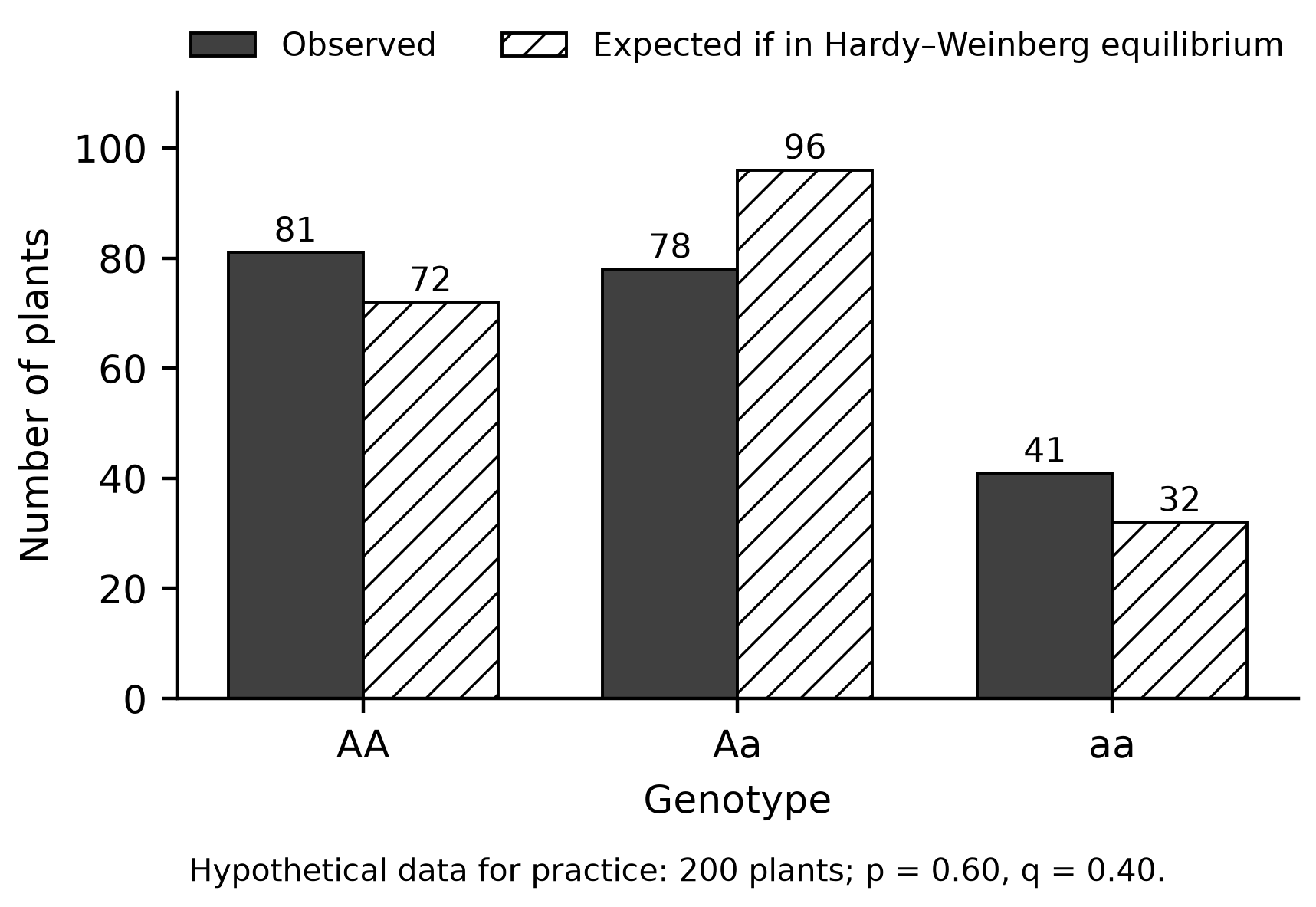
Figure 18.2. Observed genotype counts for 200 wildflowers compared with Hardy–Weinberg expectations calculated from p = 0.60.
Avoid three errors: using percentages instead of counts, taking expected values from a cross's 1 : 2 : 1 ratio instead of p², 2pq and q², and forgetting to square the deviations.
Try it 18.3. A sample of 400 fish contains 230 AA, 140 Aa and 30 aa. Test the Hardy–Weinberg null hypothesis at p = 0.05, then state what your conclusion does and does not show.
Genetic variation and a population's future
Genetic variation affects whether a population can withstand environmental change (AP Biology Course and Exam Description, topic 7.11). When a new pathogen or a warmer climate arrives, a diverse population is more likely to include individuals whose alleles let them survive and reproduce; a uniform one may include none. Because drift strips variation from small populations, a bottleneck leaves lasting risk, since lost alleles return only slowly, through mutation or gene flow.
Whether an allele helps depends on the environment: dark fur hides a desert mouse on dark lava but exposes it to predators on pale sand.
Worked example 18.5: why one blight destroyed a crop
In 1840s Ireland, farmers depended on a single potato variety. When potato blight arrived, the crop failed across the country, leading to more than a million deaths and the emigration of nearly two million people (OpenStax Biology 2e, The Importance of Biodiversity to Human Life). Solution. One variety meant one shared susceptibility, so no plant carried resistance for selection to favor.
Try it 18.4. A seed bank can store 1,000 seeds of a rare wildflower in one of two ways: all from one large population, or 100 from each of ten separate populations. Which collection better protects the species against a future disease? Justify your choice.
Check your try-it work
18.1. (a) b copies = 110 + 2(100) = 310 of 500, so q = 0.62. (b) (110 + 100)/250 = 0.84. Part (a) counts gene copies; part (b) counts individuals, so each Bb lizard counts fully in (b) although it holds one b.
18.2. (a) Drift through a bottleneck; random. (b) Drift through a founder effect; random. (c) Gene flow; not random, because it moves the field toward the neighbor's frequencies. (d) Mutation; random with respect to need.
18.3. p = (460 + 140)/800 = 0.75. Expected counts are 225 AA, 150 Aa and 25 aa. χ² = 25/225 + 100/150 + 25/25 = 0.11 + 0.67 + 1.00 = 1.78, below 3.84 and 5.99, so fail to reject. The counts are consistent with equilibrium for this gene; they do not show that all five conditions hold.
18.4. The ten-population collection. Drift, local selection and limited gene flow make separate populations carry different alleles, so sampling many captures more of the species' variation and more chances of disease resistance. One population, however large, holds only its own subset.
Practice
Under "Printed practice" after this chapter are Questions 211–224 and Written task 20, a long free-response task. Questions 211–214 share a genotype table, 215–218 a bird-population graph and 219–221 an island model. Draw the written task's graph on its printed grid. Explanations for every choice, and the task's rubric and sample response, appear under "Chapter 18: answers and explanations."
Before you move on
Without notes, write both Hardy–Weinberg equations, list the five conditions, and redo Worked example 18.4 on blank paper. In one week, redo Try it 18.3. Chapter 19 uses drift and gene flow to explain how new species form.