What to practice
- Compare graph, table and symbolic evidence for a limit
Predict before you read. A function is undefined at : can its limit at 1 exist? Another function has the value 5 at : must its limit at 1 equal 5? Write yes or no for each. Example 3.6 settles both.
This chapter reads limits from formulas, graphs, tables and sentences, and shows when one representation hides what another reveals. Chapter 4 adds the algebra that evaluates limits exactly.
Change at an instant
An average rate of change needs two times. A speedometer reports a rate at one time. Calculus joins the two ideas by sliding the second time toward the first and watching what the average rates approach. That target value is a limit.
Example 3.1: from formula to table to limit
A ball's height is meters, seconds after it is thrown (constructed practice data). Find its velocity at .
Over the interval from 1 to , the average velocity is a difference quotient. Since and ,
for every . A table of these averages, with negative and positive:
| Average velocity (m/s) | 5.5 | 5.05 | 5.005 | 4.995 | 4.95 | 4.5 |
At the quotient is , which has no value. Yet from both sides the averages close in on 5, so the velocity at is 5 meters per second:
The formula produced the table, the table pointed to 5, and the simplified formula confirmed it. Chapter 5 turns this quotient into the derivative.
Limit notation and what it does not say
The statement means that can be kept as close to as you like by taking close enough to , from both sides, with .
- One side at a time. uses inputs less than ; uses inputs greater than . The two-sided limit exists exactly when both one-sided limits exist and are equal.
- The point itself is excluded. The value may differ from the limit, or may not exist. Neither fact changes the limit.
- A limit is a number. A limit fails to exist when the outputs grow without bound, oscillate without settling, or approach different values from the two sides (course framework). Writing records how the limit fails; it does not name a value.
Common error. "The function is undefined at 3, so the limit at 3 does not exist." The limit depends only on inputs near 3, so the first fact says nothing about the second.
Read limits from graphs
On a graph, an open circle marks a point that is not on the graph, a filled dot marks the function's value, and a dashed vertical line marks a vertical asymptote. To read a one-sided limit, trace the curve toward the input from that side and report the height the curve approaches, not the height of any dot.
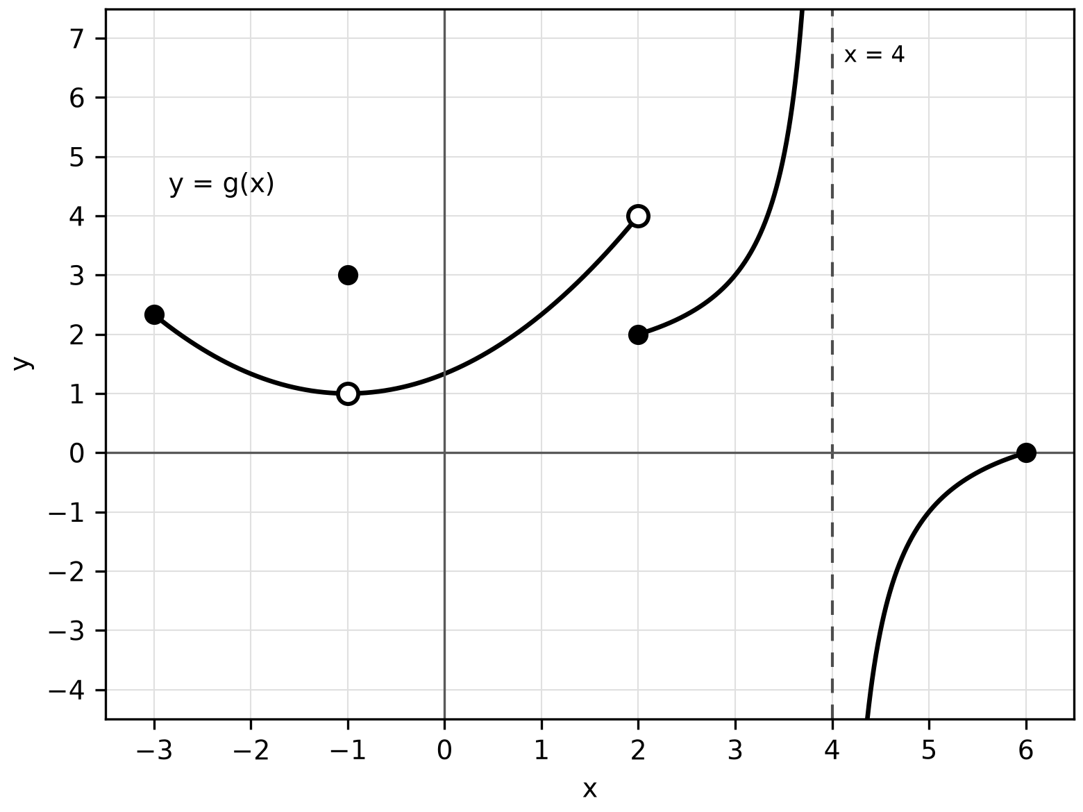
Figure 3.1. A constructed function with three different kinds of trouble.
Example 3.2: four readings from one graph
Use Figure 3.1.
- At . From both sides the curve approaches the open circle at height 1, so . The filled dot gives . The limit exists and differs from the value.
- At from the left. The curve rises toward the open circle at , so .
- At from the right. The curve starts at the filled dot , so . The one-sided limits differ, so does not exist.
- At . The outputs grow without bound from the left and decrease without bound from the right. Both one-sided limits fail to exist, and so does the two-sided limit; is a vertical asymptote.
Graphs have limited resolution. A small hole, or a jump narrower than a pixel, can disappear at a coarse scale, so treat a graph as evidence and check doubtful features with the formula.
Read limits from tables
A table shows outputs at a few chosen inputs. To estimate , choose inputs that approach from both sides and look for a value that the outputs settle toward.
Example 3.3: choose the inputs, and know when to stop
Estimate .
Substitution gives , so a table is a reasonable first method. Because appears only as , the outputs for and are equal, and one row covers both sides:
| (or ) | 0.1 | 0.01 | 0.001 |
|---|---|---|---|
| Output | 0.166620 | 0.166666 | 0.166667 |
The outputs settle near , which suggests the limit .
Now push further. At a calculator that works in double precision gives 0.166533, at it gives 0.177636, and at it gives 0; a handheld that keeps about 14 digits goes wrong even sooner. The function has not changed: the calculator subtracts two nearly equal numbers and loses digits. Stop the table once successive outputs agree to the precision you need.
Why not stop with the table? A table suggests a value and cannot prove one. Chapter 4, Example 4.2, proves that the limit is exactly with algebra. Use a table when the algebra is unclear or a question supplies data, and use algebra when a question asks for an exact value.
Use limit laws
When the separate limits exist, limits combine the way the expressions do. Suppose and .
- Sum, difference and constant multiple: the limit of is , and the limit of is .
- Product and quotient: the limit of is , and the limit of is provided that .
- Powers and roots: the limit of is , and the limit of is when .
- Composition: if is continuous at , the limit of is .
Each law needs the limits it uses to exist, and only the limits matter: the values and never enter.
Example 3.4: combine a graph with given information
The graph of has an open circle at on a smooth curve and a separate filled dot at . You are told that . Find the limit below.
The curve approaches the open circle from both sides, so . The denominator approaches , which is not 0, so the quotient law applies:
Common error. Using the dot gives . The dot is , and the laws use only limits.
Example 3.5: diagnose two incorrect claims
Claim 1. "Substituting 2 into gives , so the limit as is 0."
The quotient law requires a nonzero denominator limit, so it does not apply. A nonzero numerator over a denominator near 0 produces large outputs: at the quotient is 501, and at it is . The quotient increases without bound from the right and decreases without bound from the left, so the limit does not exist. Repair: is never 0; it signals unbounded behavior.
Claim 2. " has no limit at 0, so has no limit at 0."
Let for and for , and let . Neither has a limit at 0, but for every , so the sum has limit 0. The sum law works in one direction only: if both limits exist, the sum's limit exists. Repair: when a separate limit fails to exist, the law gives no conclusion, so simplify the combined expression first.
Connect graph, table and formula
Each representation answers a different question. The formula gives exact values and shows where trouble can occur. A table reports actual outputs near the input. A graph shows the overall behavior at one scale.
Example 3.6: three views of one function
Let for , and let .
- Formula. For , factoring gives . Near 1 the outputs are near 2.
- Table. At , 0.99, 0.999, 1.001, 1.01 and 1.1 the outputs are 1.9, 1.99, 1.999, 2.001, 2.01 and 2.1, as the formula predicts.
- Graph. Figure 3.2A shows the line with an open circle at and a filled dot at . Figure 3.2B joins sampled points the way a calculator does: it shows no hole, and the value 5 is missing.
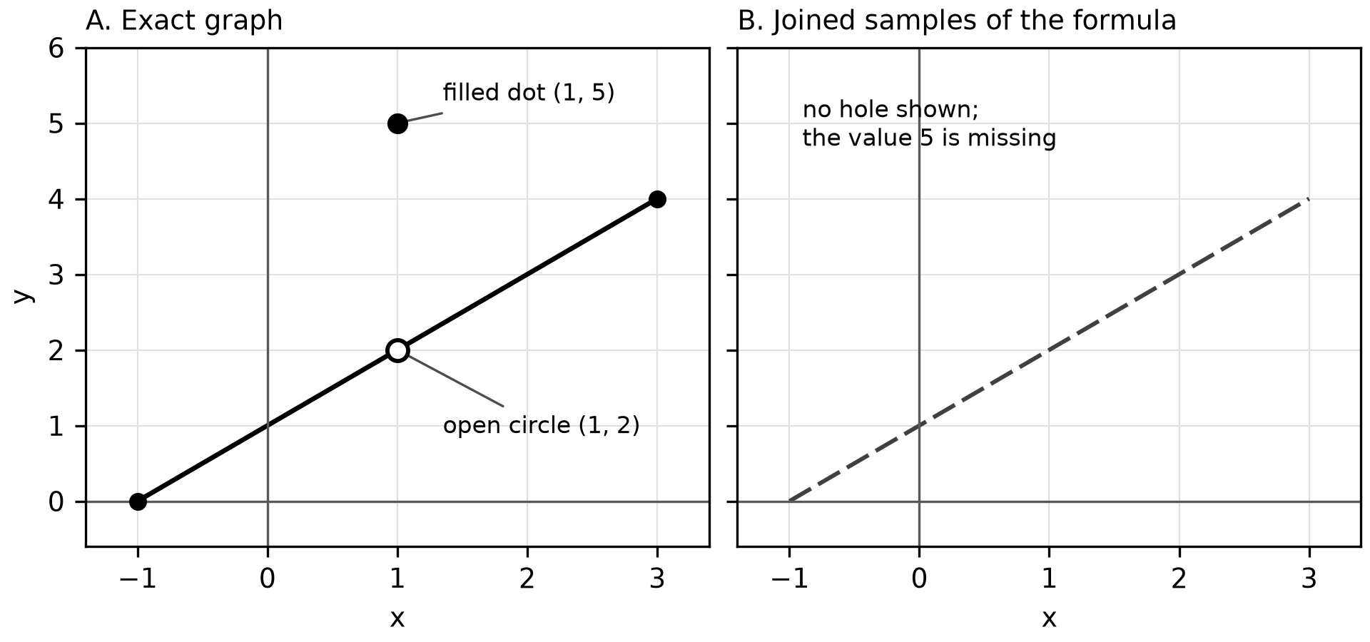
Figure 3.2. One function drawn exactly (A) and as a plotting routine draws it (B).
So while . The prediction questions now have answers: a limit can exist where the function is undefined, and the value 5 does not force the limit to be 5.
Try it
Try it 3.1. A tank holds liters at time minutes. Write the average rate of change over the interval from 2 to as a polynomial in , and find the instantaneous rate at .
Try it 3.2. Make a table of at , 0.01 and 0.001 in radian mode, then repeat in degree mode. Which estimate of is correct for calculus?
Try it 3.3. Given and , find and .
Try it 3.4. Let for , , and for . Find both one-sided limits at 3, the two-sided limit and the value .
Check your work
3.1. for . As this approaches 12 liters per minute.
3.2. Radian mode gives 0.998334, 0.999983 and 1.000000 (rounded), so the limit is 1. Degree mode gives about 0.017453 each time, which is . Calculus results such as this one hold only in radians.
3.3. , using the quotient law because the denominator limit, 3, is not 0. The root law gives .
3.4. From the left, ; from the right, . The two-sided limit is 5, and . The limit exists but differs from the value, a point Chapter 4 returns to.
Practice
Chapter 3 practice is items APCAL-C03-M01 to APCAL-C03-M14 and APCAL-C03-F01, printed after this chapter's companion panel as Questions 37–50 and Written task 1. Questions 38, 45, 46 and 50 require a graphing calculator in radian mode; the others and the written task do not. Answers, full reasoning, the error behind each wrong choice, a Repair and retry line and the written task's scoring rubric are in Answers, explanations and written responses at the back of the book, under Chapter 3: answers and explanations.
Before you move on
Close the book and write, from memory, the three ways a limit can fail to exist and one condition that the quotient law requires. Then redraw Figure 3.1 from your notes and read all four limits in Example 3.2 again. In two or three days, without the chapter, rework Example 3.4 with instead of , and check your answer with a table of your own design.