What to practice
- Check continuity conditions and choose a valid limit method
Predict before you read. After canceling a common factor, a student finds that a rational function's limit at 2 is . Is the function continuous at 2? Decide now; Example 4.4 answers it.
Chapter 3 read limits from graphs and tables. This chapter evaluates them exactly, then uses limits to define continuity, classify discontinuities, describe asymptotes and apply the Intermediate Value Theorem.
Start with substitution
Always substitute first. The result tells you what to do next.
| Substituting gives | What it means | Next step |
|---|---|---|
| A number | For a function continuous at , that number is the limit | Report it |
| Nothing yet: the form is indeterminate | Rewrite, then substitute again | |
| A nonzero number over 0 | The outputs grow without bound near | Check the sign on each side |
| No value, from a factor such as | The outputs may oscillate | Look for bounds and try the squeeze theorem |
Common error. Reporting as 0, 1 or "does not exist." The form is a signal to rewrite, not an answer.
Rewrite to remove a zero over zero
Example 4.1: factor, cancel and keep the restriction
Find .
Substitution gives . Factor:
for and . The two expressions agree at every input near , so they have the same limit: .
Write the restriction. The original function is still undefined at ; canceling changed the formula, not the function's domain.
Example 4.2: let the form choose the method
Each limit below gives , and each form signals a different rewrite.
(a) A square root in a difference: multiply by the conjugate.
(b) The same signal, with Chapter 3's table. Multiplying by gives for , so the limit as is . Example 3.3's estimate is now proved.
(c) A fraction inside a fraction: combine over a common denominator.
for , so the limit as is .
Common error. Multiplying only the numerator by the conjugate. Multiply the numerator and the denominator, or the expression changes value.
Why these choices? Factoring helps only when a polynomial has the factor . A conjugate removes a root from a difference. A common denominator clears nested fractions. When no rewrite appears, a table estimates the limit (Chapter 3), and Chapter 10 adds L'Hospital's rule for many such forms.
Squeeze a limit between bounds
Squeeze theorem. If for all near (except possibly at ) and , then .
Example 4.3: a bound that squeezes and one that does not
Find .
Substitution fails, and no algebra removes the sine. But for every , and multiplying by keeps the order:
Both bounds approach 0 as , so the limit is 0 (Figure 4.1A).
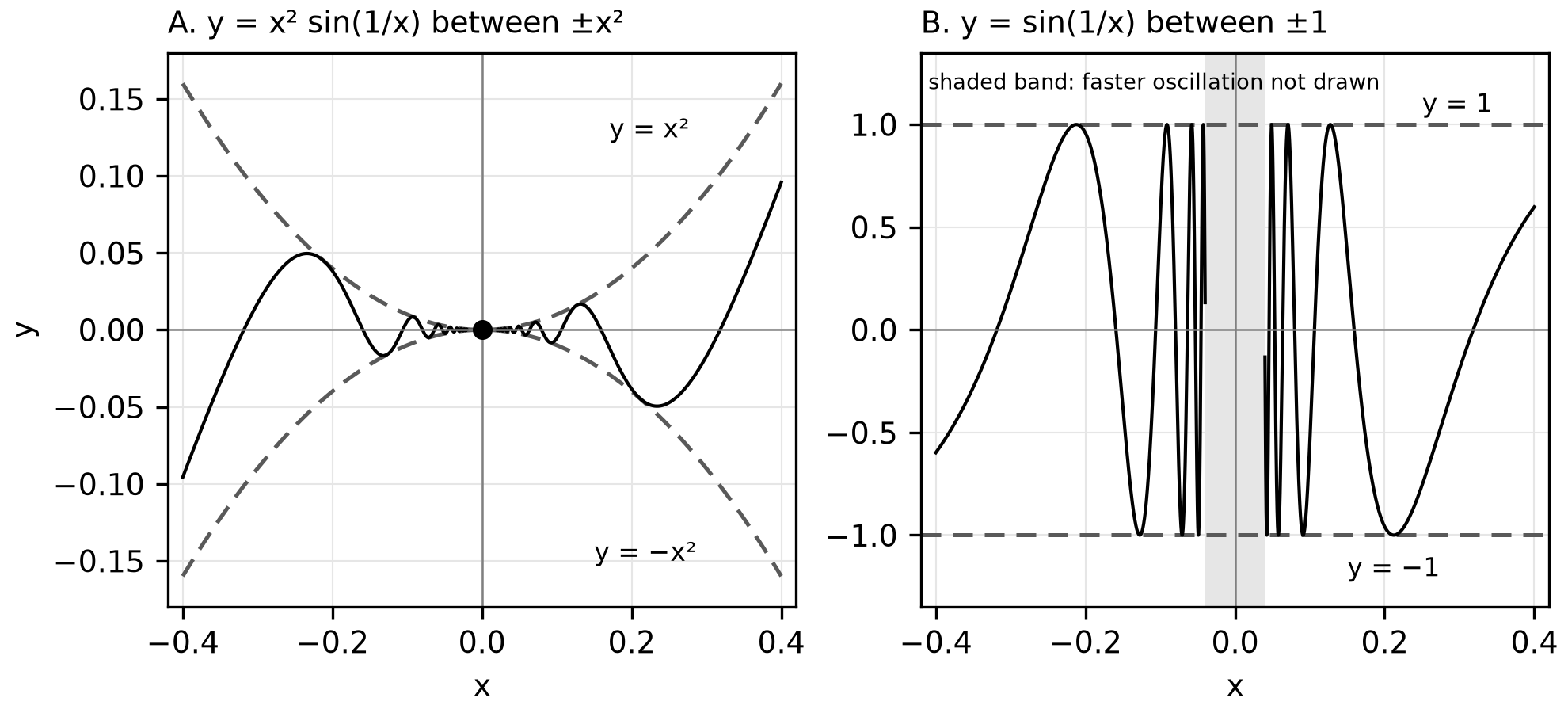
Figure 4.1. The bounds in A meet at the origin; the bounds in B never meet.
Now compare alone (Figure 4.1B). Its bounds, and 1, approach different values, so the squeeze gives no conclusion. The function reaches 1 and at inputs arbitrarily close to 0, so its limit at 0 does not exist.
The same theorem underlies two limits you will use often, valid in radians: and .
Define continuity and classify discontinuities
A function is continuous at when three conditions hold:
- is defined;
- exists;
- .
When a condition fails, the course framework names three kinds of discontinuity (course framework):
- Removable: the two-sided limit exists, but is undefined or differs from it. The graph has a hole.
- Jump: both one-sided limits exist but differ.
- Infinite (asymptotic): the outputs grow without bound on at least one side.
Example 4.4: diagnose a canceled-factor argument
Let (Figure 4.2).
Student claim. ", and is defined at 2, so is continuous at 2."
Diagnosis. Canceling is valid only for , so it shows that . It does not create a value: is , undefined. Condition 1 fails, and has a removable discontinuity at 2. Defining a new function equal to for and equal to at 2 removes it.
At both forms are undefined and the numerator does not approach 0, so the outputs are unbounded: an infinite discontinuity.
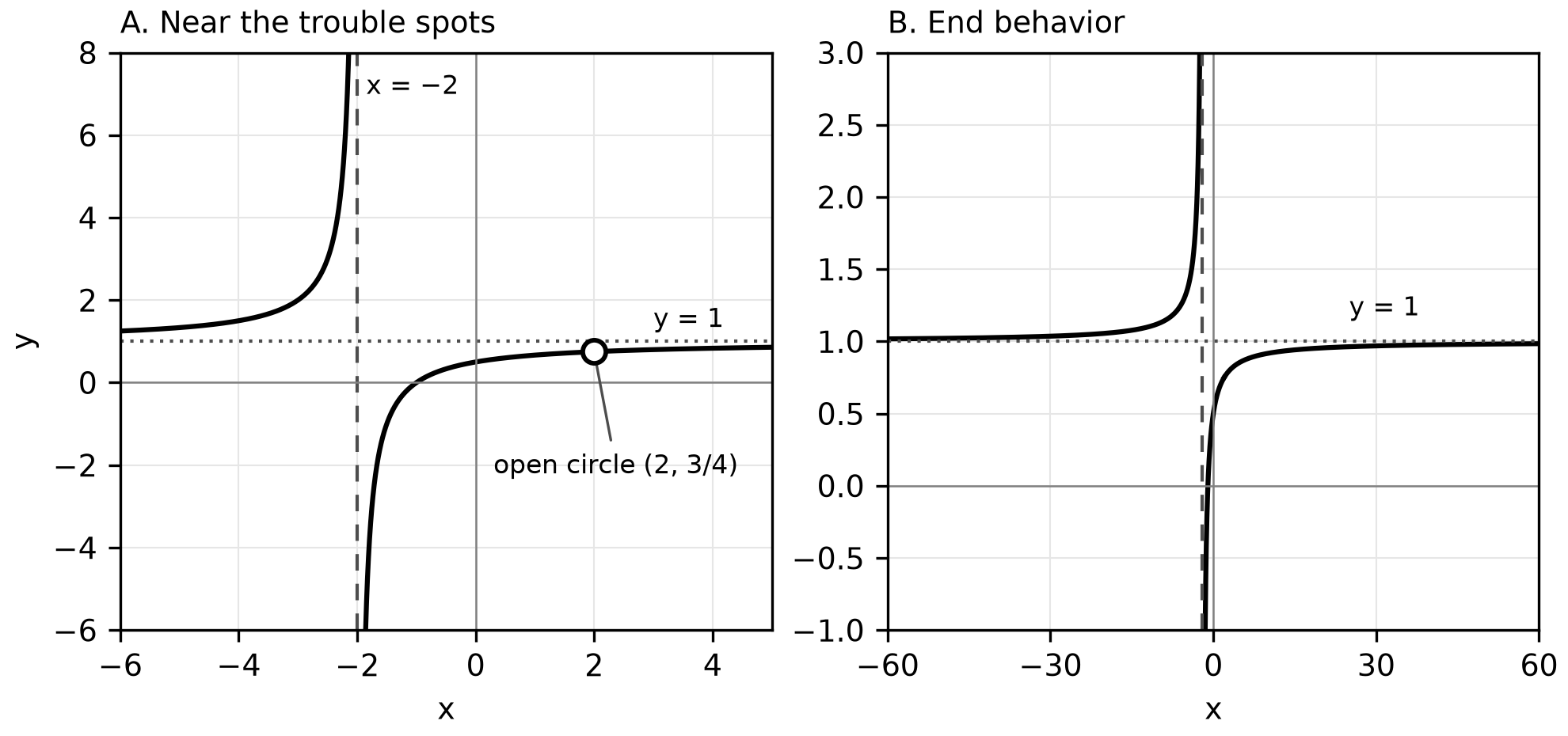
Figure 4.2. A removable discontinuity and an asymptote in one rational function (A), and its end behavior (B).
Continuity on intervals
A function is continuous on an open interval when it is continuous at every point of the interval. On a closed interval , the endpoints need only one-sided agreement: and . For example, is continuous on , though it has no inputs to the left of 1.
Polynomial, rational, power, exponential, logarithmic and trigonometric functions are continuous at every point of their domains, and so are sums, products, quotients and compositions of them. So is continuous on , and is continuous except where . For these functions, substitution gives the limit at any input in the domain.
Example 4.5: choose a constant to join two pieces
Let for and for . Find so that is continuous everywhere.
Each piece is a polynomial, so the only question is . There, and . All three conditions hold exactly when , so . Check: both one-sided limits and equal 3.
Only a removable discontinuity can be fixed by defining or redefining one value. At a jump, one value cannot equal two different one-sided limits.
Infinite limits and limits at infinity
If grows without bound as approaches from either side, the line is a vertical asymptote. If or , the line is a horizontal asymptote.
To find the direction of an infinite limit, find the sign of the numerator and the sign of the denominator on each side. A squared factor never changes sign: near , is negative on both sides, so both one-sided limits are .
For end behavior, compare the fastest-growing terms. A rational function with equal degrees approaches the ratio of the leading coefficients; with a larger denominator degree, it approaches 0; with a larger numerator degree, it has no horizontal asymptote. Exponential growth outpaces every power, so as .
Example 4.6: signs near an asymptote and two different ends
(a) Near , has numerator near . For slightly less than , the denominator is a small negative number, so the quotient is a large positive number: . From the right the denominator is small and positive, so .
(b) The numerator and denominator of both have degree 2 with leading coefficient 1, so at both ends (Figure 4.2B). The horizontal asymptote is .
(c) Find both end behaviors of . Because , divide by . For , and
For , , so the numerator becomes and . The graph has two horizontal asymptotes, and .
Common error. Writing for negative gives 2 at both ends.
Use the Intermediate Value Theorem
Intermediate Value Theorem (IVT). If is continuous on and is a number between and , then there is at least one in with .
The hypothesis is continuity on the closed interval. The conclusion guarantees existence only: it gives no location and no count.
Example 4.7: complete an IVT argument
Show that has a zero between 1 and 2.
A weak argument. " is negative and is positive, so has a zero." It never states continuity. The function on is negative at and positive at 1, yet it has no zero, because it is not continuous at 0.
A complete argument. is a polynomial, so it is continuous on . Since , the IVT gives at least one in with . A calculator locates it near , but the theorem alone does not.
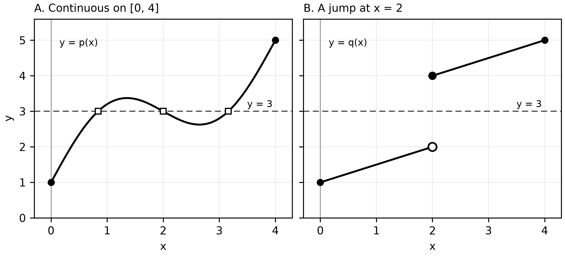
Figure 4.3. Equal endpoint values, different guarantees: a continuous function (A) and a function with a jump (B).
In Figure 4.3A the value 3 occurs three times, more than the theorem promises. In Figure 4.3B the endpoint values are the same, but the jump skips every output between 2 and 4.
Common error. Applying the IVT to a value outside the endpoint outputs. With and , the theorem says nothing about .
Write the justification
Written questions award points for the reasons, not only the answers. Match the claim to the evidence it needs.
| Claim | Write |
|---|---|
| A limit's value | The rewrite or the one-sided values, and why they agree |
| is continuous at | , the two-sided limit, and the statement that they are equal |
| The type of a discontinuity | Both one-sided limits, and if it exists |
| A vertical asymptote at | A one-sided limit that is or |
| for some | Continuity on , and , between them, then the IVT |
For example: "Because , and , the limit exists and equals , so is continuous at 2."
Try it
Try it 4.1. Find .
Try it 4.2. Let . Classify each discontinuity, give both one-sided limits at any vertical asymptote, and find the horizontal asymptote.
Try it 4.3. Let for , for , and for . Find and so that is continuous everywhere.
Try it 4.4. Show that has a solution between 0 and .
Check your work
4.1. for , so the quotient equals for , and the limit is 6.
4.2. for . At 3 there is a removable discontinuity; the limit is . At the numerator approaches 1, so and : an infinite discontinuity. Equal degrees give the horizontal asymptote .
4.3. At 1: , so . At 2: , so .
4.4. Let , continuous on as a difference of continuous functions. Since and , the IVT gives a between 0 and with , that is, . (A calculator gives .)
Practice
Chapter 4 practice is items APCAL-C04-M01 to APCAL-C04-M15 and the written tasks APCAL-C04-F01 and APCAL-C04-F02. They are printed after this chapter's companion panel as Questions 51–65 and Written tasks 2 and 3. Questions 58, 63, 64 and 65 and Written task 3 require a graphing calculator in radian mode; the others do not. Answers, full reasoning, the error behind each wrong choice, a Repair and retry line and both scoring rubrics are in Answers, explanations and written responses at the back of the book, under Chapter 4: answers and explanations.
Before you move on
From memory, write the substitution table, the three continuity conditions and the hypothesis of the IVT. Then explain, in two sentences, why canceling a factor never makes a function continuous. In two or three days, without notes, rework Example 4.5 with for , and redo Example 4.6(c) for .