What to practice
- Translate a rate statement and check a proposed solution or slope field
Predict before you read. Every segment of a slope field is horizontal along the line . Is a solution of that differential equation? Write yes or no and one reason. Example 17.4 settles it.
This chapter turns rate statements into differential equations, checks proposed solutions, and reads the behavior of solutions from a slope field without solving anything. Chapter 18 adds the algebra that produces solution formulas.
Equations about rates
A differential equation relates a function to its derivatives (course framework). In , the unknown is a function of , and the equation describes its slope at every point. A solution is a function, not a number: substituting it makes the equation true for every in an interval.
A differential equation may have infinitely many solutions, as does. It need not: forces both squares to be 0, so its only solution is , and has no real solution at all. An initial condition such as picks out one particular solution.
Translate a rate statement
Turn a sentence into an equation one phrase at a time. "Rate of change of " becomes . "Proportional to" means "equals a constant times." "Decreases" fixes the sign of the right side. Whatever the rate depends on goes on the right side.
Example 17.1: three statements, three equations
Each quantity depends on time .
| Statement | Equation | What the sign of says |
|---|---|---|
| A population grows at a rate proportional to its size. | , because the population grows. | |
| A cup's temperature changes at a rate proportional to the difference between and the room temperature of 20 degrees. | : a cup hotter than the room has and must cool. | |
| The depth of water in a draining tank decreases at a rate proportional to the square root of the depth. | , with the minus sign written in. |
The second row shows the method at work. Read "the difference between and 20" as , then decide the sign of from the physical situation, not from the wording alone.
Common error. Writing for "proportional to ." A constant added to is not a constant multiple of .
Verify a proposed solution
To check that a function solves a differential equation, compute its derivative, substitute the function and its derivative into the equation, and simplify. The two sides must agree for every in an interval, not at one convenient point. Check any initial condition separately.
Example 17.2: verify a solution and see a family
Show that solves with .
The left side is . The right side is . The sides agree for every , and . The function is the particular solution.
Replace 2 by any constant . Then has derivative , and , so every member of this family is a solution. Choosing gives the line , a solution whose slope is 1 everywhere.
Example 17.3: diagnose an incorrect verification
A student checks whether solves with :
". Also , so at , , and . They match, so it is a solution."
The initial condition is satisfied, but the equation was tested at only one point. Substitute everywhere: . The difference is 0 only at , so the function is not a solution. At , for example, while . Repair: subtract the right side from , simplify symbolically, and show that the difference is 0 for every .
Draw a slope field
A slope field draws, at each point of a grid, a short segment whose slope is the value of there. It represents the differential equation on a finite set of points (course framework). A solution curve is tangent to the segment at every grid point it passes through.
Example 17.4: from a table of slopes to a field
For , the slope at each integer point is :
| 0 | |||||
| 0 | 1 | ||||
| 0 | 1 | 2 | |||
| 0 | 1 | 2 | 3 |
Each diagonal of the table repeats one value, because the slope depends only on . Figure 17.1 draws the same equation on a grid with spacing one half.
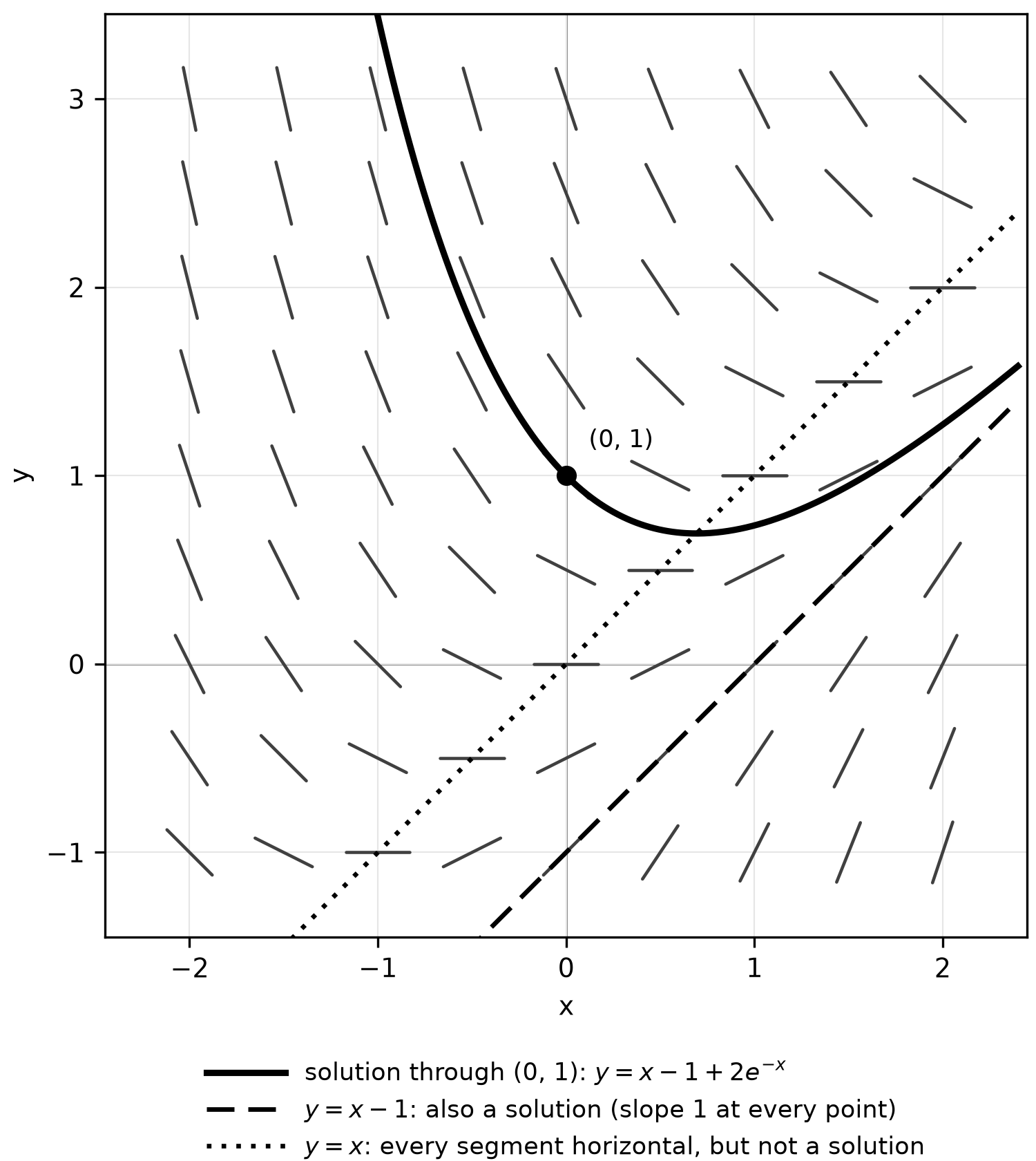
Figure 17.1. Slope field for , with the solution through and two lines.
Now answer the opening question. Along every segment is horizontal, but the line itself has slope 1, so a curve that followed it would cross the segments instead of following them: is not a solution. Along every segment has slope , which is the line's own slope, so that line is a solution, as Example 17.2 found.
Read a slope field: choose the test
Matching a field to an equation is fastest with tests chosen in this order:
- Where are the segments horizontal? The zero-slope locus of each candidate is easy to find, and one look at the field often eliminates several candidates at once.
- What does the slope depend on? If the segments are parallel along every horizontal line, the slope depends only on . If they are parallel along every vertical line, it depends only on .
- What is the sign in one region? One point usually decides between equations that differ only in sign.
Example 17.5: match a field to its equation
Which equation could Figure 17.1 show: , , or ?
Start with zero slopes, because that test separates the most candidates. The field is horizontal along . For the zero locus is , and for it is the two axes, so both are eliminated. The other two equations share the zero locus , so test a sign. At the segment falls, with slope ; gives there and gives 1. The field shows .
Why not compute slopes at many points? Random checks take longer and can miss a sign difference. Two well-chosen tests settle this match.
Equilibrium solutions and sign regions
If the right side of is 0 at , then the constant function is a solution: its derivative is 0 and the equation gives 0. Such a horizontal-line solution is an equilibrium solution. Unlike the line above, it really is a solution, because a horizontal line has slope 0. Where solutions increase; where they decrease.
Example 17.6: read a cooling model without solving it
A bowl of soup cools in a 20-degree room according to , with in degrees Celsius and in minutes (constructed practice data). Figure 17.2 shows the slope field.
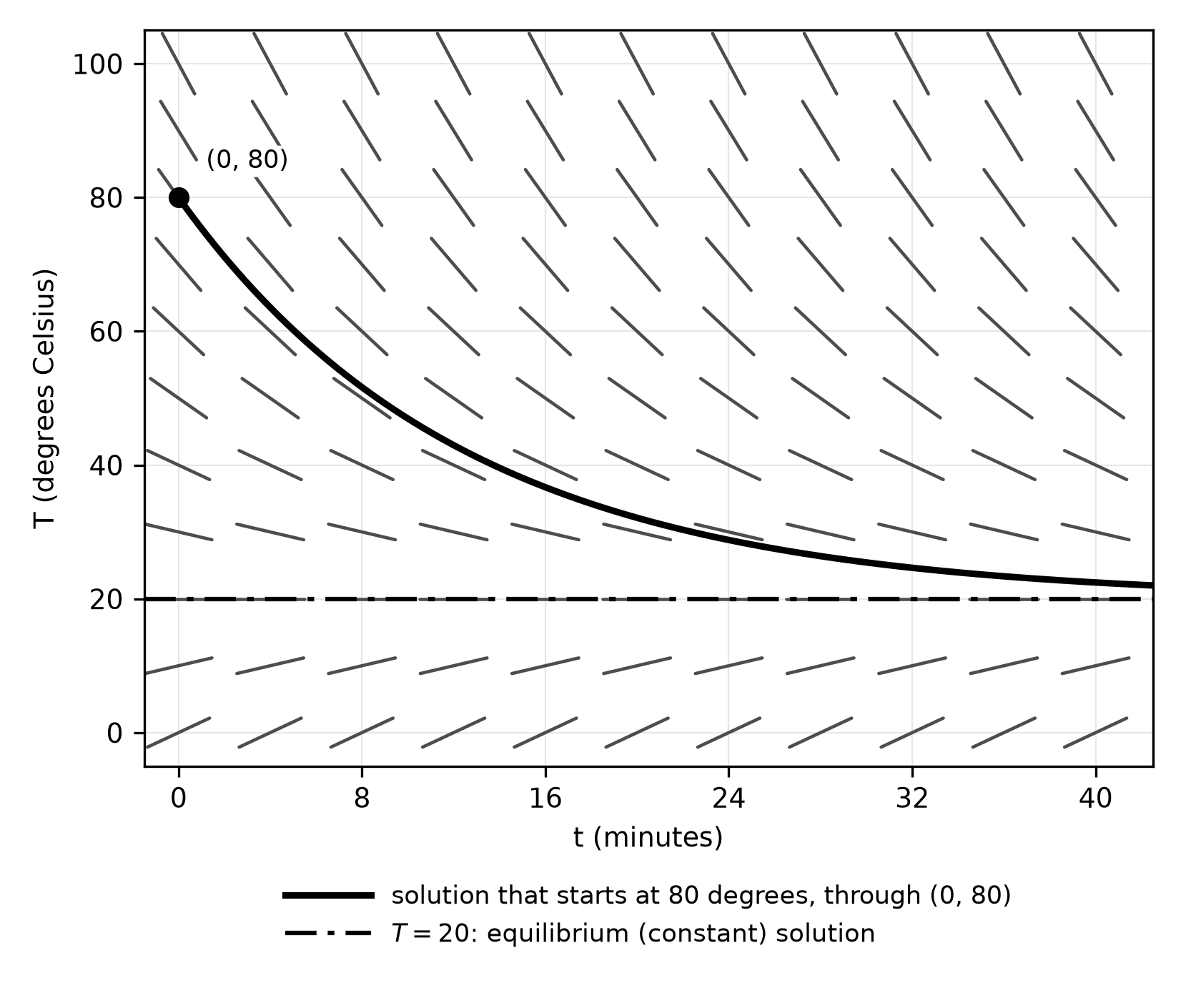
Figure 17.2. Slope field for , with the solution that starts at 80 degrees.
- Rates. At the rate is degrees per minute. At it is , and at it is .
- Equilibrium. makes the rate 0, so is a solution: soup at room temperature stays there.
- Signs. Above 20 the temperature falls; below 20 it rises. Either way it moves toward 20.
- Concavity. Differentiating the equation with respect to gives , which is positive above 20. The cooling curve is concave up, so the soup cools more slowly as time passes.
- No crossing. Because the right side is differentiable, only one particular solution passes through a given point (course framework). If the soup's curve reached 20, two different solutions would share a point, so the soup approaches room temperature without going below it.
The field answered every question here graphically. Chapter 18 derives the formula and finds .
Example 17.7: concavity and a tangent-line estimate
Let be the solution of with . Estimate and decide whether the estimate is too large or too small.
At the slope is , so the tangent line is and . Differentiate the equation, remembering that depends on : . At this is , so the graph is concave up near and lies above its tangent line. The estimate 0.8 is an underestimate. (The exact value, from Example 17.2, is .)
Common error. Treating as a constant gives . The derivative of is , which must be replaced by .
Try it
Try it 17.1. The fish population of a lake grows at a rate proportional to , and fishing removes 400 fish per year. Write a differential equation for , with in years.
Try it 17.2. Both and satisfy . Which, if either, solves ?
Try it 17.3. For , find the equilibrium solution, the values of for which solutions increase, and the concavity of solutions with .
Try it 17.4. For , find the slope at each of the nine points with and in , and describe the segments you would draw.
Check your work
17.1. with . Growth contributes ; harvesting subtracts a constant 400 per year.
17.2. For : and , so it is a solution. For : but , which never agree. Only the first solves the equation.
17.3. . Solutions increase for and decrease for , so they move away from 40. , so solutions with are concave up.
17.4. The slope is 0 at all five points on the axes, 1 at and , and at and . Draw horizontal segments on the axes, segments at 45 degrees rising in the first and third quadrants, and segments falling in the second and fourth.
Practice
Chapter 17 practice is items APCAL-C17-M01 to APCAL-C17-M07 and the written task APCAL-C17-F01. They are printed after this chapter's companion panel as Questions 226–232 and Written task 24. Questions 226 and 232 require a graphing calculator in radian mode; the others and the written task do not. Answers, full reasoning, the error behind each wrong choice, a Repair and retry line and the written task's scoring rubric are in Answers, explanations and written responses at the back of the book, under Chapter 17: answers and explanations.
Before you move on
Close the book and write, from memory, the three tests for matching a slope field and why the zero-slope test comes first. Then sketch the slope field for at nine points and mark the line that is a solution. In two or three days, without the chapter, rework Example 17.6 for a cold drink at 5 degrees in a 25-degree room with , and check your signs against Try it 17.3.