What to practice
- Apply initial conditions, preserve equilibrium solutions and interpret domains
Predict before you read. The function solves with . The formula gives at . Is the point on this particular solution? Write yes or no. Example 18.3 settles it.
Chapter 17 read solutions from equations and slope fields. This chapter finds solution formulas by separation of variables, states the interval on which each particular solution lives, and applies the results to exponential growth and decay.
When separation applies
Some differential equations can be solved by separation of variables, and antidifferentiation then produces a general solution (course framework). The method needs the right side to factor as , a function of times a function of :
- is separable, with and .
- is separable, because .
- is not separable: a sum does not factor into an part times a part.
Figure 18.1 lays out the procedure. Step 2 is the one most often skipped.
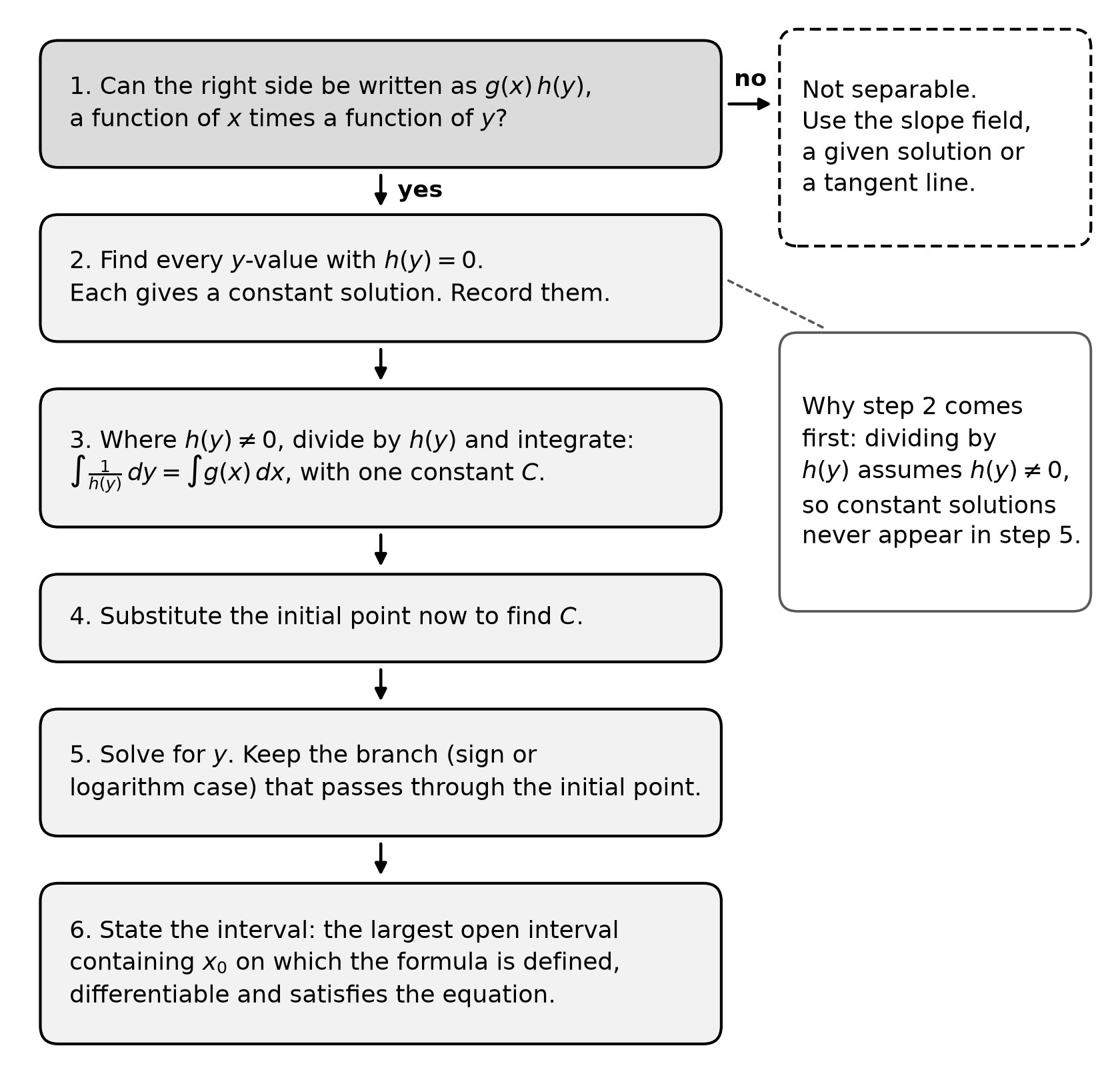
Figure 18.1. Six steps for solving .
Example 18.1: a general solution and a particular solution
Solve with .
- Constant solutions. is 0 at , so is a solution.
- Separate and integrate. For : , so .
- Find the constant now. At : , so .
- Solve for . . At the initial point , so .
- Interval. The formula is defined and differentiable for every real .
Check: and . The general solution is for any constant ; restores the constant solution that dividing by set aside.
Why find before solving for ? With the logarithm still in place, one substitution gives , and the sign of at the initial point removes the absolute value. Solving first creates a that must be sorted out later.
Particular solutions live on intervals
A general solution may describe infinitely many solutions. The course framework adds that only one particular solution passes through a given point. That holds for every equation in this chapter's examples, whose right sides are differentiable near each initial point, but it can fail where the right side is not differentiable: from Chapter 17 has two solutions through a point where , the constant and a tank that empties at that moment. Solutions may also be subject to domain restrictions (course framework). A particular solution is a differentiable function on one open interval that contains the initial input.
To find that interval, list every input that the formula or the equation cannot accept: a zero denominator, the even root of a negative number, the logarithm of a number that is not positive, or a point where is undefined. Remove those inputs and keep the single open interval that contains the initial input. Any other part of the formula's domain belongs to other solutions, even where the formula still satisfies the equation.
Example 18.2: choose the branch
Solve with .
Separate: , so . At : , so and . Two branches satisfy this, and . The initial value is negative, so . Check: , which equals because .
Interval: the equation divides by , so cannot be 0, and the root requires . The solution lives on , roughly . At the formula gives , where is undefined.
Example 18.3: a solution that stops
Solve with .
The constant solution is . For : , so . At , , so .
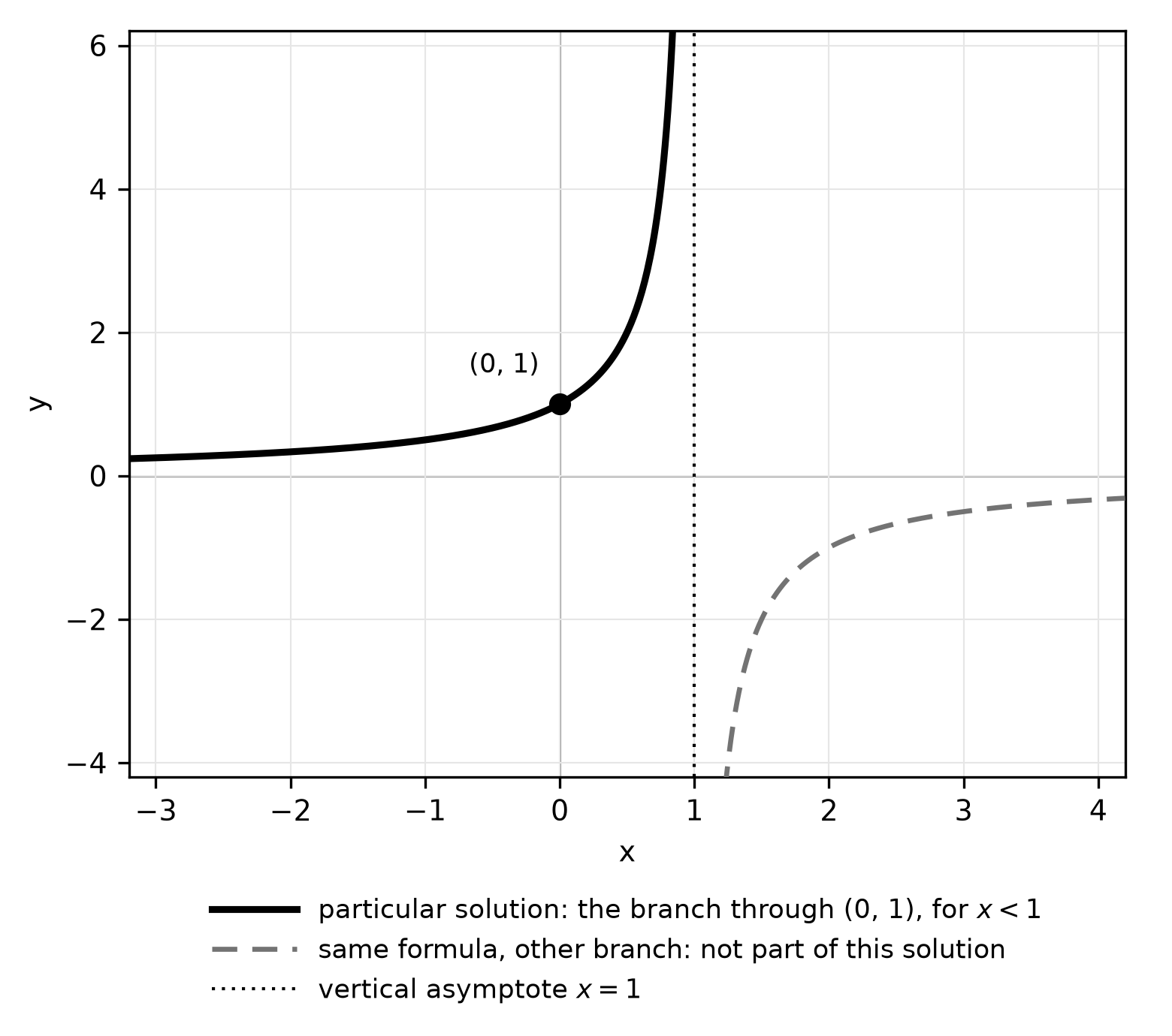
Figure 18.2. The formula has two branches; the particular solution is only the branch through .
The formula is undefined at , and increases without bound as . The particular solution is the solid branch on . The dashed branch also satisfies , but it is a different solution, the one through . So the answer to the opening question is no: the formula's value at does not belong to this solution.
Common error. Reporting the domain as "all ." A solution must be differentiable on one interval through the initial point, so the answer is .
Example 18.4: when the antiderivative has no formula
Solve with , and find .
No elementary antiderivative exists, so write the solution as an accumulation function:
By the Fundamental Theorem of Calculus, , and . With a calculator, . The representation changed from formula to integral, and the solution is still exact.
Exponential models
"The rate of change of a quantity is proportional to the size of the quantity" translates to . Separating gives , and with the solution is . When the quantity grows; when it decays. The same model covers motion along a line, such as a velocity that satisfies .
Over equal time steps an exponential quantity is multiplied by the same factor . A table with a constant ratio of successive values fits this model; a constant difference fits a linear one. The doubling time is for growth, and the half-life is for decay.
Common error. Reading "grows 5% per year" as . That phrase gives a yearly factor of 1.05, so and . The equation describes a different model, one whose yearly factor is .
Example 18.5: half-life from a description
A dose of 80 mg of a medication leaves the body at a rate proportional to the amount present and halves every 5 hours (constructed practice data). Find the amount after 12 hours and the rate at 10 hours.
From , . So , which also equals . After two half-lives mg, and mg. At , , so the amount is decreasing at about 2.773 mg per hour.
A linear model that loses 8 mg per hour matches the first 5 hours but predicts 0 mg at 10 hours and mg at 12 hours, which is impossible. The proportional model removes the same fraction, not the same amount, in each 5-hour period.
Example 18.6: test a table for an exponential model
A culture is counted every 2 hours (constructed practice data).
| (hours) | 0 | 2 | 4 | 6 |
|---|---|---|---|---|
| (thousands of cells) | 500 | 600 | 720 | 864 |
The differences are 100, 120 and 144, so a linear model does not fit. The ratios are , the same over each 2-hour step, so fits with , which gives per hour. The model predicts thousand cells. It satisfies , so at the culture grows at about thousand cells per hour. The table, a list of numbers, became a differential equation and a formula.
Example 18.7: motion along a line
A boat coasts with its engine off. Its velocity satisfies , with in meters per second and in seconds, and (constructed practice data). The model gives : the velocity halves every seconds and never reaches 0. In the first 4 seconds the boat travels meters. After seconds it has traveled meters, which is always less than 24.
Example 18.8: a shifted exponential
Chapter 17, Example 17.6, read the cooling model from its slope field. Solve it with .
The constant solution is . For : , so . At , , so . Then degrees, and when , at minutes.
The formula confirms what Chapter 17 read from the field: the temperature decreases, the graph is concave up, and the curve approaches 20 without crossing it. With any starting temperature , the same steps give . Figure 18.3 shows three cases.
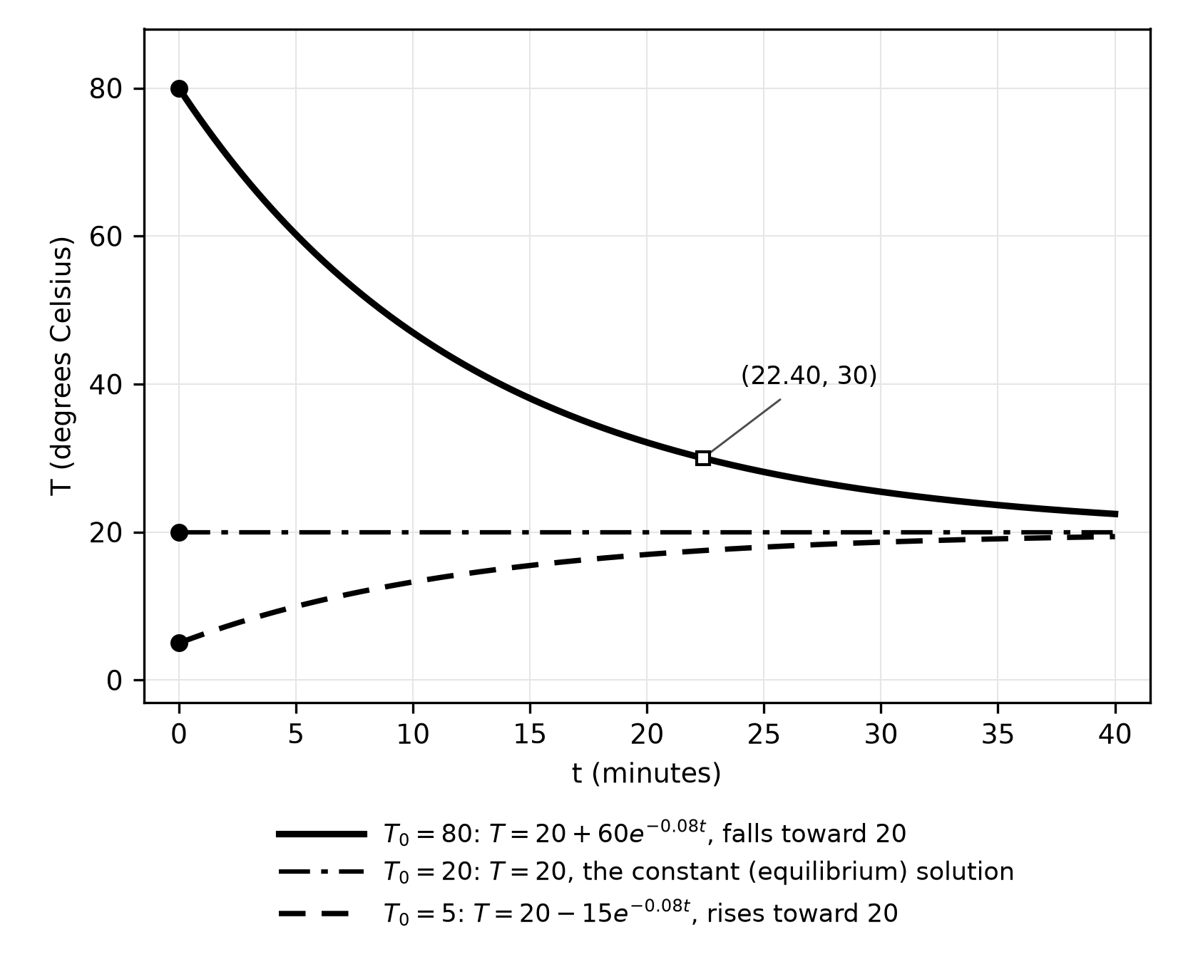
Figure 18.3. Particular solutions of for starting temperatures 80, 20 and 5 degrees Celsius, shown for minutes.
Diagnose incorrect solutions
Example 18.9: the constant in the wrong place
A student solves with :
", so and . Then gives , so ."
Check by substitution: , but . The two differ by , so the answer fails. The constant belongs with the antiderivatives, before exponentiating: , so , and . Then gives , and . The division by also set aside the constant solution , which is .
Common error. Adding after exponentiating. An additive constant on the logarithm becomes a multiplying constant on .
Try it
Try it 18.1. Solve with , and state the interval of the solution.
Try it 18.2. A population grows at a rate proportional to its size and doubles every 9 years. How long does it take to triple?
Try it 18.3. Solve with (Try it 17.3 described its slope field), and find when .
Try it 18.4. For , find the particular solutions with and with .
Check your work
18.1. gives , and gives . So and . The logarithm needs , so the solution lives on .
18.2. , and gives years.
18.3. . Then gives .
18.4. For : with , so for all . For the solution is the constant , which the division by would have lost.
Practice
Chapter 18 practice is items APCAL-C18-M01 to APCAL-C18-M09 and the written tasks APCAL-C18-F01 and APCAL-C18-F02. They are printed after this chapter's companion panel as Questions 233–241 and Written tasks 25 and 26. Questions 239, 240 and 241 and Written task 26 require a graphing calculator in radian mode; the others and Written task 25 do not. Answers, full reasoning, the error behind each wrong choice, a Repair and retry line and the written tasks' scoring rubrics are in Answers, explanations and written responses at the back of the book, under Chapter 18: answers and explanations.
Before you move on
Close the book and redraw Figure 18.1 from memory, including the reason step 2 comes before the division. Then solve Example 18.1 again with and state its interval. In two or three days, without the chapter, rework Example 18.5 for a 120 mg dose with a 6-hour half-life, and explain in one sentence why a linear model fails.