What to practice
- Separate accumulated change, final amount, average value and distance
Unit 8 asks what an integral means. This chapter covers topics 8.1 to 8.3 of the course framework: average value, motion along a line, and accumulation in context. Most lost points here come from computing a correct integral that answers a different question.
One rate, five questions
Let be the rate at which a quantity changes, for . Five common questions use the same rate in five different ways.
| Question | Setup | Units |
|---|---|---|
| By how much did change? | units of | |
| How much is there at time ? | units of | |
| How much change happened, counting increases and decreases alike? | units of | |
| What is the average value of ? | units of | |
| What is the average rate of change of ? | units of per unit of |
Before you integrate, name the row. The first two rows differ only by the starting amount. The third row needs an absolute value. The last two rows look alike but average different functions: the average value averages itself, while the average rate of change averages its rate.
Average value: an equal-area rectangle
Sample a continuous function at equally spaced points of , with spacing . The ordinary average of the samples is
The sum on the right is a Riemann sum, so as grows the sample average approaches the average value
Multiply both sides by : a rectangle of height on has the same signed area as the region under . Because is continuous, it has a minimum and a maximum on , lies between them, and takes every value in between, so for at least one in . This is the Mean Value Theorem for integrals; it guarantees that such a exists, not where it is.
Worked example 19.1: three different averages
A drone's height is meters for minutes. Find its average height, its average rate of change of height, and the times when it is at its average height.
Average height. Integrate the height itself:
meters.
Average rate of change. meters per minute. The drone ends where it started, although it spent the whole flight in the air.
When is it at 6 meters? Solve : , so , about 1.268 and 4.732 minutes.
The tempting shortcut, averaging the endpoint heights, gives meters, which is wrong: endpoint averaging is reliable only for linear functions. Figure 19.1 shows why 6 is right.
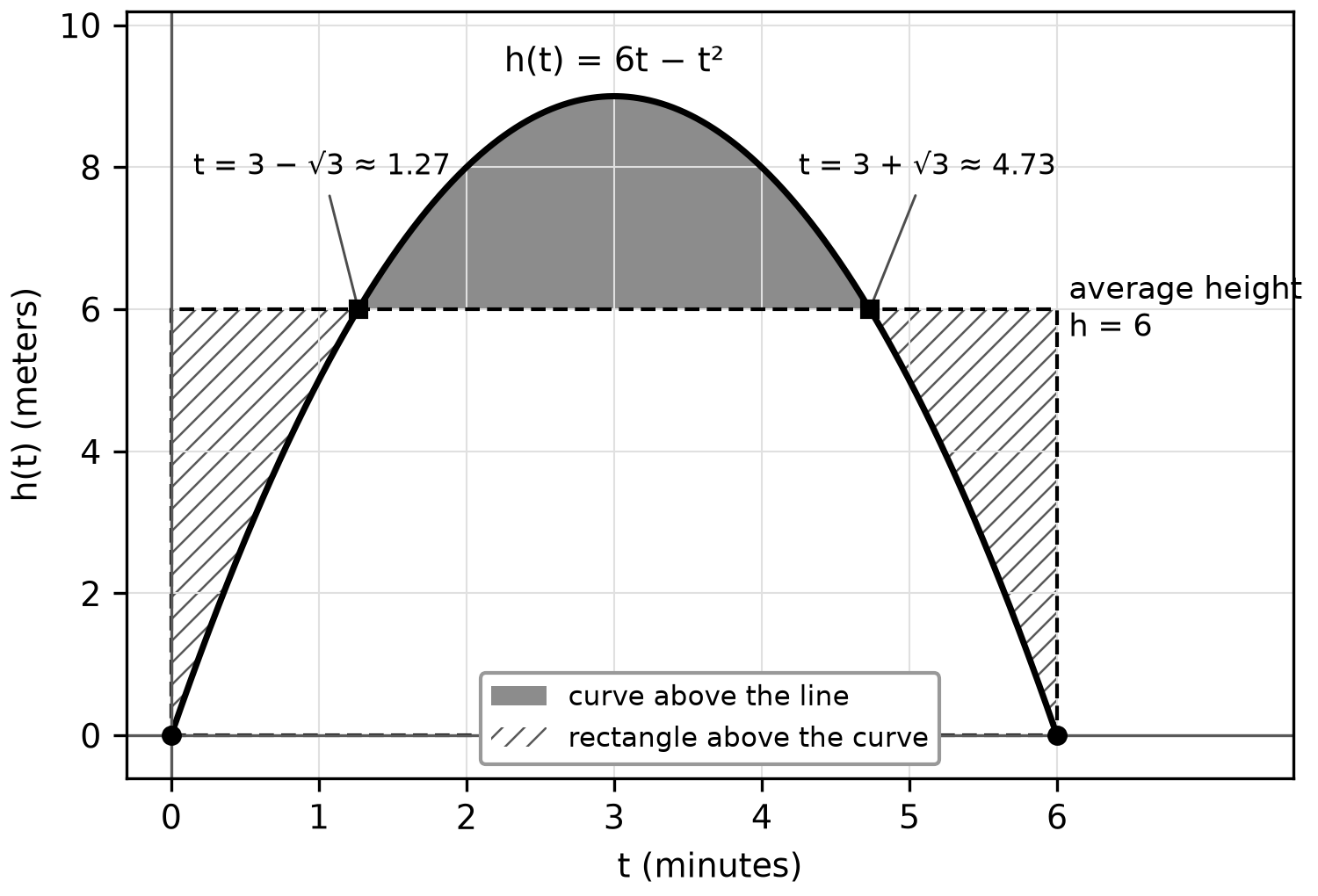
Figure 19.1. The dark region above the line has the same area as the two hatched corners of the rectangle, so the rectangle of height 6 on matches the area under the arch.
Displacement, distance and position
For a particle moving along a line with velocity :
- Displacement on is . Leftward motion counts as negative.
- Total distance traveled is , the integral of speed.
- Position at time is .
The same pattern links acceleration to velocity: .
Worked example 19.2: read signed areas from a velocity graph
A particle moves with meters per second for , and . Find its displacement, its distance traveled and .
Velocity is positive on , negative on and positive on . With the antiderivative , the three integrals are 4, and 4 (Figure 19.2, panel A).
- Displacement: meters.
- Distance: meters (panel B).
- Position: .
Track the trip to check: , and . The particle moved 4 meters right, 4 left and 4 right again; it had already reached once, at . Divide each total by 4 seconds. The average velocity is 1 meter per second, but the average speed is 3 meters per second.
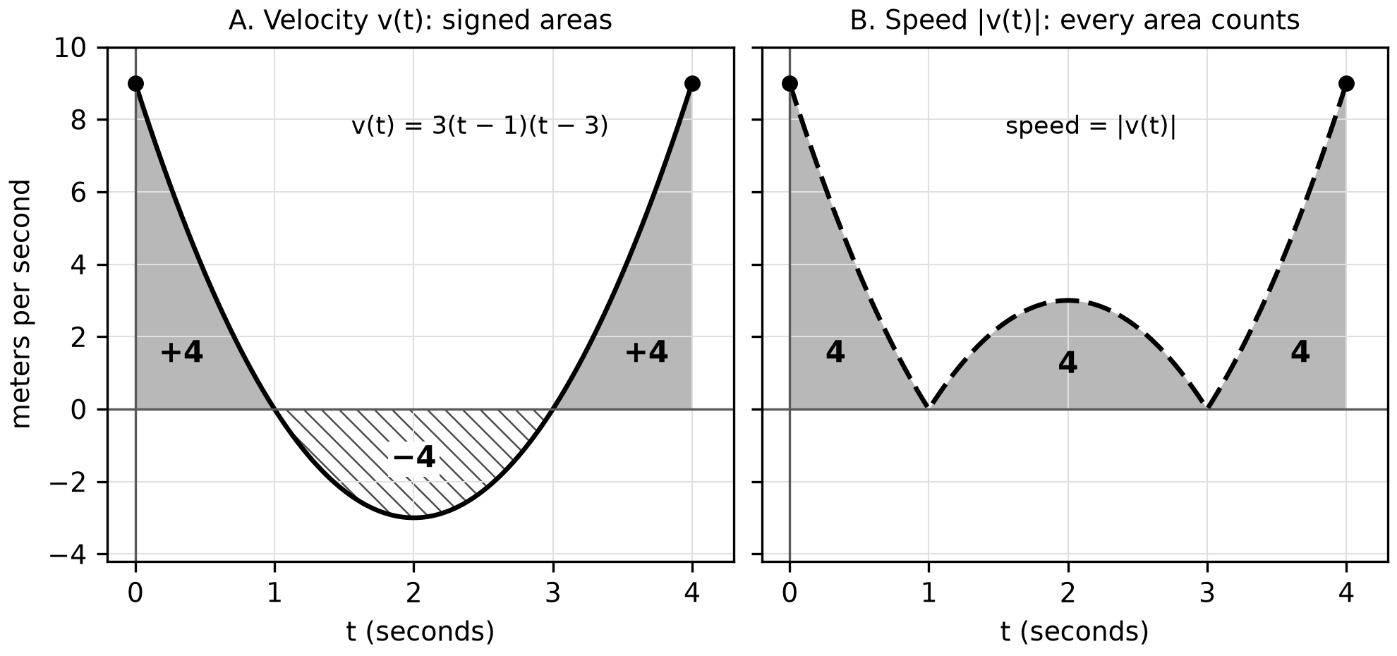
Figure 19.2. The velocity's signed areas (A) give displacement. The speed's areas (B) give distance.
Worked example 19.3: choose how to find distance
Find the distance traveled on when .
Method choice. Without a calculator, split at the zero of . Here is negative on and positive on , so
and the distance is , while the displacement is 0. With a calculator, enter directly; that avoids finding the zero but still requires the absolute value. A single signed integral, here 0, is never a distance unless keeps one sign.
Net change in applied contexts
When something enters at rate and leaves at rate , the amount present is
and . The amount rises exactly when inflow exceeds outflow, even if inflow itself is falling. Keep three graphs apart in your mind: the inflow rate, the outflow rate and the amount. A peak on a rate graph is not a peak in the amount. Rate units times time units give amount units; liters per minute times minutes give liters.
Worked example 19.4: estimate an amount from a rate table
A home battery stores 20 kilowatt-hours (kWh) at noon. It charges at power kilowatts, where is hours after noon (constructed practice data):
| (hours) | 0 | 0.5 | 1.5 | 2 |
|---|---|---|---|---|
| (kilowatts) | 6.0 | 7.2 | 5.6 | 3.2 |
Representation change. The table becomes trapezoids, and the trapezoids estimate an integral. The intervals have unequal widths, so use each width:
So kWh, because kilowatts times hours give kilowatt-hours, and the battery holds about kWh at 2 p.m. The table says nothing about concavity between the readings, so you cannot tell whether 11.9 overestimates or underestimates.
Worked example 19.5: inflow, outflow and the greatest amount
A tank holds 100 liters at . Water enters at and leaves at liters per minute for . When is the amount greatest, and what is it?
The net rate is , which is zero at , positive before and negative after (Figure 19.3, panel A). So
Check the critical point and both endpoints:
| (minutes) | 0 | 6 | 10 |
|---|---|---|---|
| (liters) | 100 | 208 | 160 |
The greatest amount is 208 liters, at . Over the whole interval, liters entered and liters left, a net gain of 60 liters.
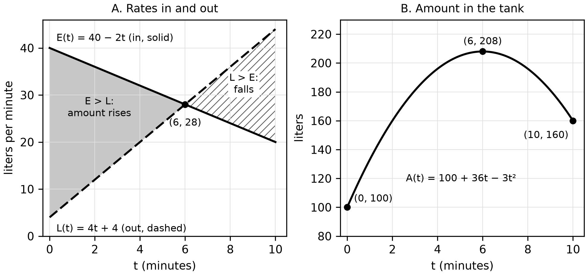
Figure 19.3. Where inflow exceeds outflow (A), the amount rises (B). The amount peaks where the rate graphs cross.
Worked example 19.6: diagnose a flawed solution
Task: for the tank in Example 19.5, find the amount at , justify when the amount is greatest, and find how much water entered. One student wrote:
"(i) , so the tank holds 60 liters. (ii) The amount is greatest at because there. (iii) So 60 liters of water flowed in."
- (i) The integral is the change in the amount, not the amount. Repair: liters.
- (ii) A zero of only makes a candidate. Repair: state that changes from positive to negative there, or compare the three values in the table.
- (iii) Net change is not inflow. Repair: 300 liters flowed in and 240 flowed out.
Errors (i) and (iii) answer a nearby question from the five-row table; error (ii) skips part of a justification. Log (i) and (iii) as OBJECT and (ii) as CONDITION.
Try it
Try it 19.1. For on , find the average value, the average rate of change, and the value guaranteed by the Mean Value Theorem for integrals.
Try it 19.2. A particle moves with meters per second for , and . Find its displacement, its distance traveled and .
Try it 19.3. A yard holds 50 tons of gravel at . Trucks deliver 12 tons per hour, and a loader removes gravel at tons per hour, for hours. Find the greatest amount in the yard, the amount at , and the gravel removed.
Check your work
19.1. . The average rate of change is . Solve : , which lies in .
19.2. meters. Velocity is negative on and positive on : and , so the distance is meters. .
19.3. The net rate is , zero at , positive before and negative after. With , the candidates give , and , so the greatest amount is 74 tons, at . The loader removed tons.
Retrieve and review
- In two days. Without looking, rewrite the five-row table. Then redo Example 19.5 with outflow . You should find a greatest amount of 200 liters, at .
- In one week. Rework any question below that you missed, and log its code: OBJECT for answering a different row of the table, SIGN for a dropped negative area, UNITS for a missing or wrong unit.
- Before Chapter 20. Areas between curves reuse this chapter's idea of a signed integral: you will again decide when signs should cancel and when they should not.
Practice
Chapter 19's practice is items APCAL-C19-M01 to APCAL-C19-M11 and the written task APCAL-C19-F01, printed after this chapter's companion panel as Questions 242–252 and Written task 27. Questions 242–248 are no-calculator work. Questions 249–252 and Written task 27 require a graphing calculator in radian mode; give decimals to the nearest thousandth. Answers, the error behind each wrong choice, the rubric and a complete response are in Answers, explanations and written responses, under Chapter 19: answers and explanations.