What to practice
- Connect inputs, outputs, domains, graphs, tables, average change and linear/quadratic patterns.
Start with two climbs that look the same
A drone and a weather balloon both leave the ground and both reach 40 meters exactly 20 seconds later. Over those 20 seconds each climbed at an average of 2 meters per second. Yet the drone rose quickly at first and slowly near the top, while the balloon did the reverse. One number cannot tell them apart. A description of how the rate itself changes can.
This chapter builds that description. You will state what a function promises, read direction and zeros from a graph, compute and interpret average rates of change, and use the pattern of those rates to separate linear from quadratic behavior. It covers topics 1.1 to 1.3 of the AP Precalculus Course and Exam Description.
What a function promises
A function is a rule that assigns each input exactly one output. The set of inputs is the domain; the set of outputs the function actually produces is the range. The input variable is the independent variable, and the output variable is the dependent variable. When , the output 7 is the image of the input 3, and 3 belongs to the preimage of 7. An output can have several inputs in its preimage, but an input never has two outputs.
Two functions are equal only when they have the same domain and give the same output for every input in it (CED clarifications and corrections). Matching formulas are not enough. If is defined only for , 2, 3 and 4, while is defined for all real , then and are different functions even though they agree wherever both are defined.
Worked example 3.1: read a table as a function
A coffee cart records the number of customers waiting, , at hours after opening (constructed practice data).
| (hours) | 0 | 1 | 2 | 3 | 4 |
|---|---|---|---|---|---|
| (customers) | 2 | 6 | 6 | 3 | 0 |
Is a function of ? Yes. Each input appears once with one output. Repeated outputs are allowed.
Domain and range. The table defines only at , 1, 2, 3 and 4, so that set is the domain. The range is the set of outputs, .
Image and preimage. The image of 3 is . The preimage of 6 is , because both inputs produce 6. Do not stop at the first match.
Reverse the roles. Is a function of ? No. The value would need two different outputs, 1 and 2.
Read direction, zeros and sign from a graph
A function is increasing on an interval if, for all and in the interval with , . It is decreasing if always gives . The phrase "for all" matters: comparing only the endpoints of an interval proves nothing about the inputs in between. Whether an interval of increase is written with open or closed ends is not assessed on the exam; this book uses open intervals.
A zero of is an input where ; on the graph it is an -intercept. Where the graph is above the -axis the function is positive, and where it is below, negative. Direction and sign are separate features. A function can be decreasing while positive and increasing while negative.
Worked example 3.2: read a graph completely
Figure 3.1 shows on the closed domain .
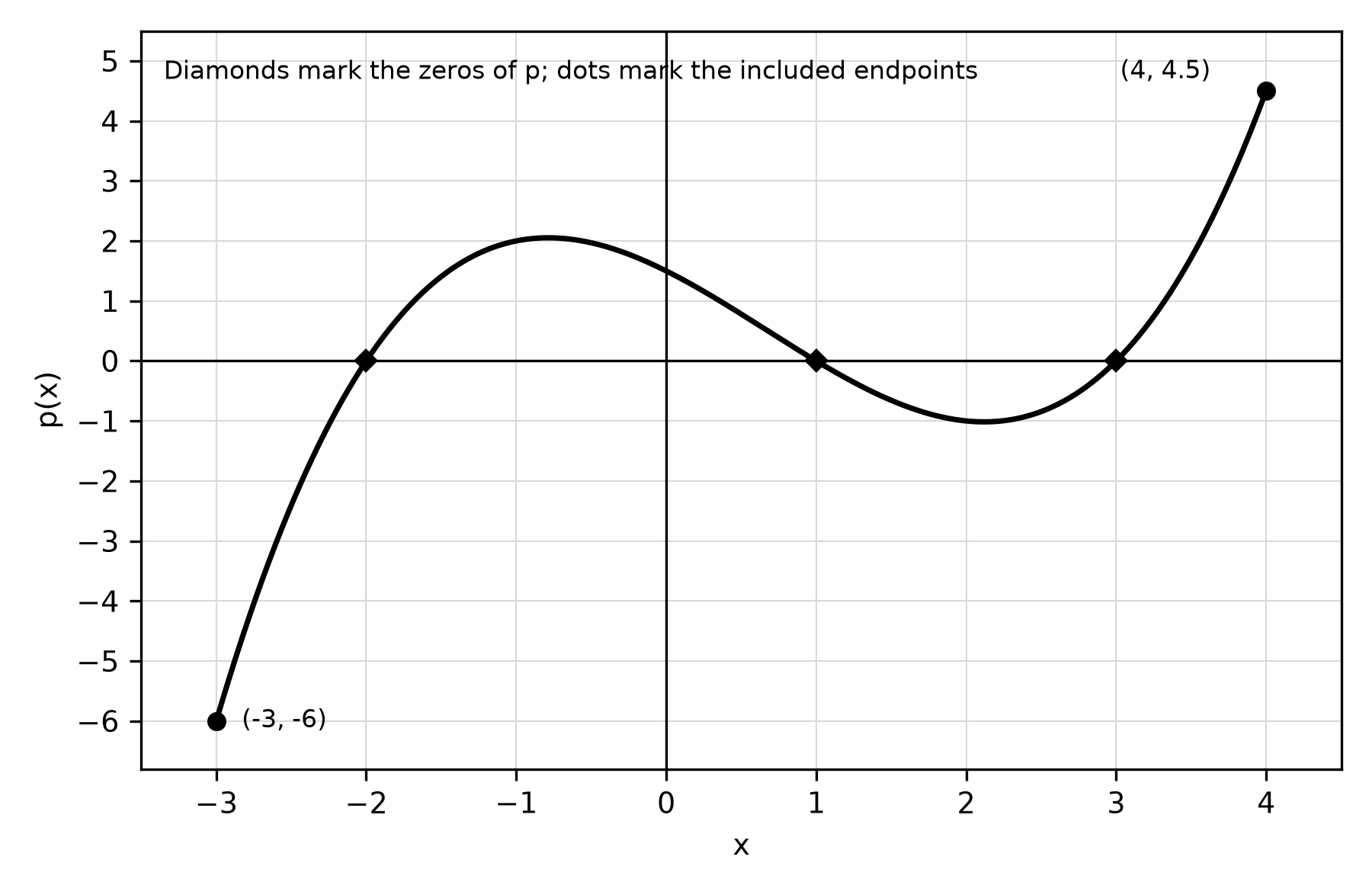
Figure 3.1. Direction and sign are separate: decreases on both sides of its zero at .
Zeros. The graph meets the axis at , 1 and 3, matching the factors.
Sign. on and on ; on and on . The endpoint is included, so the bracket is closed there.
Direction. increases on about , decreases on about , and increases on . The turning inputs are estimates read from the graph.
Range. The lowest output is at the left endpoint and the highest is 4.5 at the right endpoint, since the peak near 2 and the low point near lie between them. The range is .
Build a graph from a description
Rates of change describe shape. A graph is concave up on an interval where its rate of change is increasing and concave down where its rate of change is decreasing. A rising graph that rises more and more slowly is concave down; a falling graph that falls more and more slowly is concave up.
Worked example 3.3: sketch a flight
A drone takes off at seconds. It climbs quickly at first and then more slowly, reaching 40 meters at 20 seconds. It hovers until 35 seconds and then descends at a steady 1.6 meters per second until it lands. Sketch altitude against time.
Fix the known points. Plot , and . The descent takes seconds, so the drone lands at .
Match each phrase to a shape. "Quickly, then more slowly" means positive rates that decrease: rising and concave down. "Hovers" means a rate of 0, a horizontal segment. "Steady descent" means a constant negative rate, a straight segment with slope .
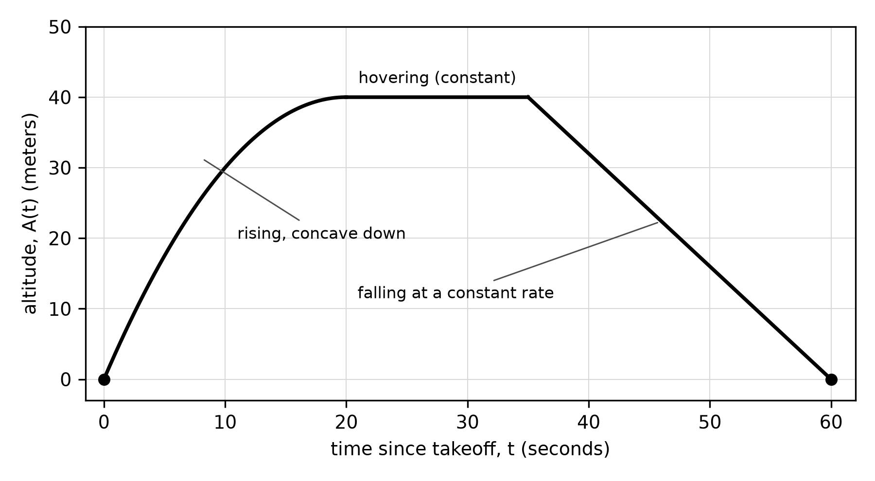
Figure 3.2. A graph built from words (constructed practice data, not a measured flight).
The opening balloon, which rose slowly and then quickly, would be rising and concave up on the same interval.
Average rate of change
The average rate of change of over the interval is
and its units are output units per input unit. It is the constant rate that would produce the same change in output over the interval. Geometrically, it is the slope of the secant line through and .
The sign carries meaning. A positive average rate means the output ended higher than it began: the two quantities changed in the same direction. A negative average rate means one quantity increased while the other decreased. The average rate says nothing about what happened inside the interval.
Worked example 3.4: compare rates over unequal steps
A cyclist's distance from home is recorded at three times (constructed practice data).
| (hours) | 0 | 2 | 5 |
|---|---|---|---|
| (kilometers) | 3 | 9 | 18 |
The output changes are 6 and 9, which look different. The rates are and kilometers per hour, and over the rate is as well. When steps are unequal, compare rates, not raw changes. These data are consistent with the linear function , but three points cannot prove that the cyclist rode steadily between them.
Worked example 3.5: estimate a rate at a point
The rate of change at a single input is approximated by average rates over smaller and smaller intervals that contain it. Let . From , the secants to , 4 and 3 have slopes , and (Figure 3.3).
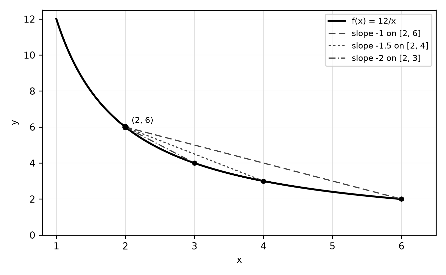
Figure 3.3. Shorter secants from give better estimates of the rate at .
Shrink further. Over the rate is , and over it is . The rate at lies between these, about . Repeating at gives about on and on , so the rate there is about . The function is decreasing at both inputs but decreasing four times faster at .
Linear and quadratic patterns of change
A linear function has the same average rate of change over every interval, so its rates change at a rate of 0. For a quadratic function, the average rates over consecutive equal-length intervals change by a constant amount: they follow a linear pattern. When those rates increase, the graph is concave up; when they decrease, it is concave down.
Worked example 3.6: a tossed ball
A ball's height is meters, seconds after it is tossed. Use half-second steps for , while the ball is still in the air.
| 0 | 0.5 | 1 | 1.5 | 2 | 2.5 | |
|---|---|---|---|---|---|---|
| 2 | 7.75 | 11 | 11.75 | 10 | 5.75 |
The average rates over the five intervals are 11.5, 6.5, 1.5, and meters per second. Each is 5 less than the one before, so the rates change at a constant meters per second per second. That constant change is the quadratic signature, and the decreasing rates make concave down (Figure 3.4). The ball rises, then falls, but the rate falls the whole time.
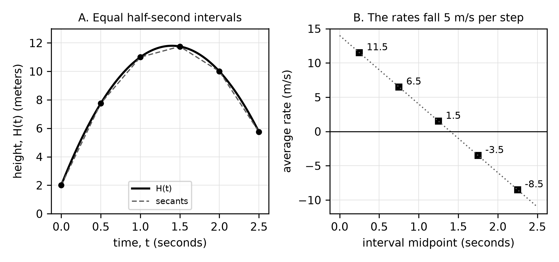
Figure 3.4. Average rates of a quadratic over equal steps form a linear pattern (constructed practice data).
Worked example 3.7: rebuild a quadratic from its rates
A quadratic has , and its average rates over , and are 5, 3 and 1. Find .
Step 1: outputs. Each interval has length 1, so each rate is an output change: , , .
Step 2: coefficients. Write . Then , and . Subtracting twice the second equation from the third gives , so and .
Step 3: check. gives .
Over unit steps, consecutive rates of differ by . Here they drop by 2, so , not .
Keep three claims separate
Many errors come from blending three different claims.
- Value: what is, and whether it is positive.
- Direction: whether is increasing or decreasing on an interval.
- Rate pattern: how fast changes, and whether that rate is increasing (concave up) or decreasing (concave down).
Worked example 3.8: repair an overreaching claim
For a function , the values at , 2, 4 and 6 are 1, 5, 3 and 7. A student writes: "The average rate of change over is , which is positive, so is increasing on ."
The arithmetic is right; the conclusion is not. Increasing requires for all , but while . So decreases somewhere between 2 and 4. A correct claim is narrower: " exceeds by 6, an average increase of 1 unit of output per unit of input."
Use a calculator for change, then interpret
On calculator-required questions, the calculator does the arithmetic; you decide what the numbers mean. A reliable routine:
- Enter the function and set the window to the stated domain.
- Use the table or value feature for outputs, then form the rate yourself.
- Estimate a rate at with a small symmetric interval such as .
- Solve with the intersect feature, and discard solutions outside the domain.
- Round only the final answer, to three decimal places unless told otherwise, and attach units.
To find a quadratic through three given points, use quadratic regression or solve a system of three equations. Linear regression returns a line, not the quadratic.
Worked example 3.9: a tank's changing depth
The water depth in a test tank is modeled by centimeters, minutes after a valve opens, for (constructed practice data).
Average rate over . and , so the rate is centimeter per minute.
Rate at . Over the calculator gives centimeters per minute. The depth is falling at even though it rose on average over .
When is the depth 15 centimeters? Graph and and use intersect three times: , and minutes. All three lie in the domain, so all three count. Stopping after the first intersection loses solutions.
Common errors to repair
- Treating a negative output as evidence of decreasing. Repair: compare outputs at two inputs.
- Calling a function increasing because one endpoint is higher. Repair: check every pair, or find a counterexample.
- Comparing raw changes over unequal steps. Repair: divide by the step.
- Forgetting the denominator , or reversing the ratio. Repair: write output change over input change.
- Using the change in rates as the leading coefficient. Repair: over unit steps it equals .
Try it
Work these on paper before reading the solutions.
- For , find the average rates over , , , and . Describe the pattern, the concavity and where decreases.
- For , simplify the average rate of change over , where .
- Are and from the section on what a function promises equal? Give the preimage of 4 under each.
- A greenhouse warms from 12 degrees Celsius at 6:00 to 27 degrees Celsius at 11:00. Find and interpret the average rate, then name one thing it does not tell you.
- Calculator: for in Worked example 3.9, estimate the rate at with . Is the depth increasing there? Are the rates increasing or decreasing near ?
Check your try-it work
- The rates are , , 1, 3 and 5. They increase by 2 each step, so is concave up everywhere, including on where it decreases. decreases for .
- and , so the rate is . If you got , you skipped the division.
- No. Their domains differ. Under , the preimage of 4 is ; under , it is , because is not in the domain of .
- degrees Celsius per hour: a steady 3 degrees per hour would produce the same total change. It does not say whether the warming was steady or whether the temperature ever fell.
- About 1.440 centimeters per minute, so the depth is increasing at . Rates near and are about 2.340 and 0.660, so the rates are decreasing and the graph is concave down there.
Review and retrieval
Close the book and write, from memory, the definition of increasing, the formula for an average rate of change with its units, and the rate pattern that identifies a quadratic. Tomorrow, rework Worked example 3.8 with the values 1, 5, 3, 7 replaced by 1, 2, 4, 7 and decide whether the student's conclusion could then be true. In about a week, redo Worked example 3.6 with one-second steps and confirm the rates still change by a constant amount. Chapter 4 uses rates to locate extrema and inflection points, Chapter 7 links constant change to arithmetic sequences, and Chapters 18 and 19 refine the calculator routine and written justification.
Practice
Twenty multiple-choice questions, Questions 31–50, and one free-response task, Written task 1, follow this chapter under Printed practice. Answer the first thirteen, Questions 31–43, without a calculator. The last seven, Questions 44–50, and Written task 1 require a graphing calculator; it is a six-point task with two pages of response space. Keys, the reasoning for every choice, the scoring guide and a sample response are under Chapter 3: answers and explanations in the answers section. Each explanation ends with a repair step that names the section of this chapter to revisit.