What to practice
- Connect finite change, factors, real/complex zeros, multiplicity and end behavior.
Let the formula predict the graph
A polynomial graph is smooth and unbroken, yet it shows where the outputs rise and fall, where the rate of change switches, where the graph crosses or only touches the -axis, and what happens far from the origin. Most of this is visible in the formula before you draw anything. This chapter covers topics 1.4 to 1.6 of the AP Precalculus Course and Exam Description. The habit to build: read the degree, the leading term and the factors first, then use a graph or a calculator to confirm what the structure predicts.
Prerequisite check. Expand ; you should get . Factor ; you should get . If either is slow, review factoring first.
Read a polynomial's structure
A polynomial function of degree can be written as
where is a nonnegative integer, every coefficient is a real number and . The term is the leading term and is the leading coefficient. A nonzero constant function has degree 0. Expressions such as , and are not polynomials, because a polynomial's variable has only nonnegative integer exponents.
Find the leading term from the highest power, not from the term written first. For , the leading term is , so the degree is 5 and the leading coefficient is 2. In factored form, multiply only the leading parts of the factors: has leading term .
Describe how the outputs change
A function is increasing on an interval if, for any inputs in that interval, ; it is decreasing if instead. A local maximum is an output at least as large as every output at nearby inputs, and a local minimum is an output no larger than every output at nearby inputs. A global (absolute) maximum or minimum is the greatest or least output on the entire domain. Three facts organize the search:
- Where a polynomial switches between increasing and decreasing, or at an included endpoint of a restricted domain, it has a local maximum or minimum.
- Between two distinct real zeros, a polynomial has at least one local maximum or local minimum, because the graph must turn around to return to the axis.
- A polynomial of even degree on all real numbers has a global maximum (when ) or a global minimum (when ). One of odd degree has neither.
The rate of change can itself increase or decrease. Where the rate of change is increasing, the graph is concave up; where it is decreasing, the graph is concave down. A point of inflection is where the rate of change switches between increasing and decreasing. Keep the two ideas separate: a function can be decreasing while its rate of change is increasing, which means the outputs fall by smaller amounts each step.
This book writes intervals of increase and decrease as open intervals. The Fall 2026 clarifications to the course framework state that discriminating between open and closed intervals for increase or decrease is outside the scope of the course and exam. Extrema at endpoints remain in scope.
Worked example 4.1: extrema on a restricted domain
Let on (Figure 4.1). Evaluate the candidates: , , and . The graph decreases on , increases on and decreases on .
- At the included endpoint , the outputs drop immediately to the right, so is a local maximum.
- At , the graph switches from decreasing to increasing: a local minimum of .
- At , it switches from increasing to decreasing: a local maximum of 10.
- At the included endpoint , the outputs just to the left are greater than 3, so is a local minimum.
Now compare. The global maximum is 19, at the endpoint , and the global minimum is , at . Checking only turning points would wrongly give 10. At the marked point of inflection, near , the rate of change stops increasing and starts decreasing.
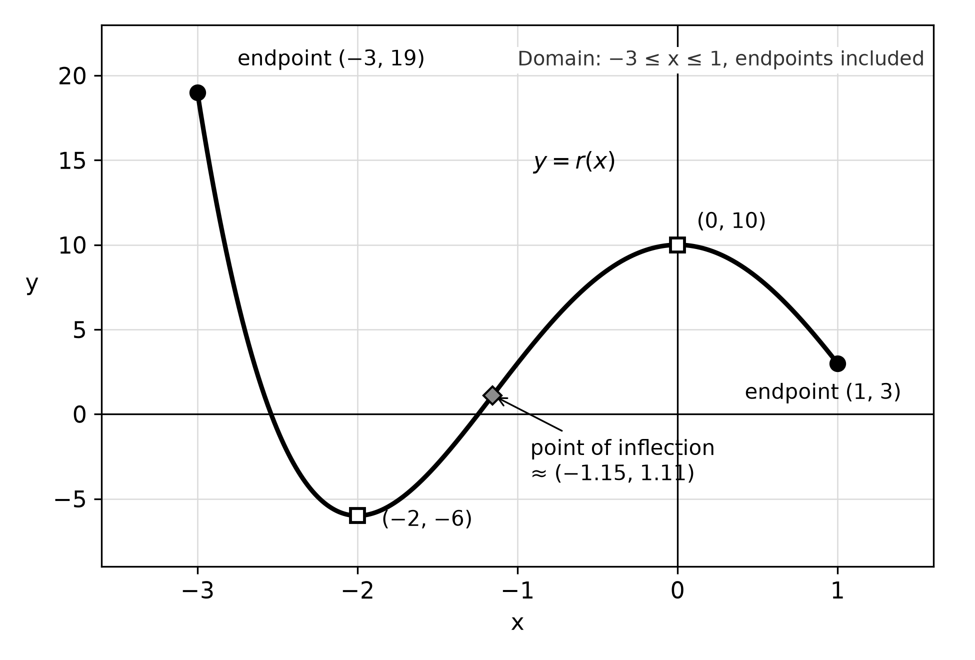
Figure 4.1. Included endpoints are candidates for extrema; here the left endpoint, not a turning point, gives the global maximum.
Worked example 4.2: read rates of change from a table
The table gives values of a polynomial at equally spaced inputs (constructed practice data).
| 0 | 1 | 2 | 3 | 4 | |
|---|---|---|---|---|---|
| 30 | 16 | 8 | 4 | 2 |
The average rates of change over the four intervals are , , and . Every rate is negative, so decreases over each interval. The rates themselves increase, so the outputs fall by less each step, which is consistent with a graph that is decreasing and concave up. Read the two features separately: the signs of the rates give increasing or decreasing, and the changes in the rates give concavity. A table is evidence only over the intervals it shows; it cannot reveal what happens between rows.
Try it 4.1. Let on . Its only turning point in that domain is . List every local extremum, then the global maximum and minimum.
Zeros, factors and multiplicity
If is a real zero of , then is a factor of and is an -intercept of the graph. A polynomial of degree has exactly complex zeros when each is counted by its multiplicity. When the coefficients are real, nonreal zeros come in conjugate pairs: if is a zero, so is .
If is a factor but is not, the zero has multiplicity . Multiplicity controls what the graph does at the zero:
- Odd multiplicity: the sign of changes, so the graph crosses the axis. At multiplicity 3 or more, it flattens as it crosses.
- Even multiplicity: the sign does not change, so the graph touches the axis and turns back, tangent to it.
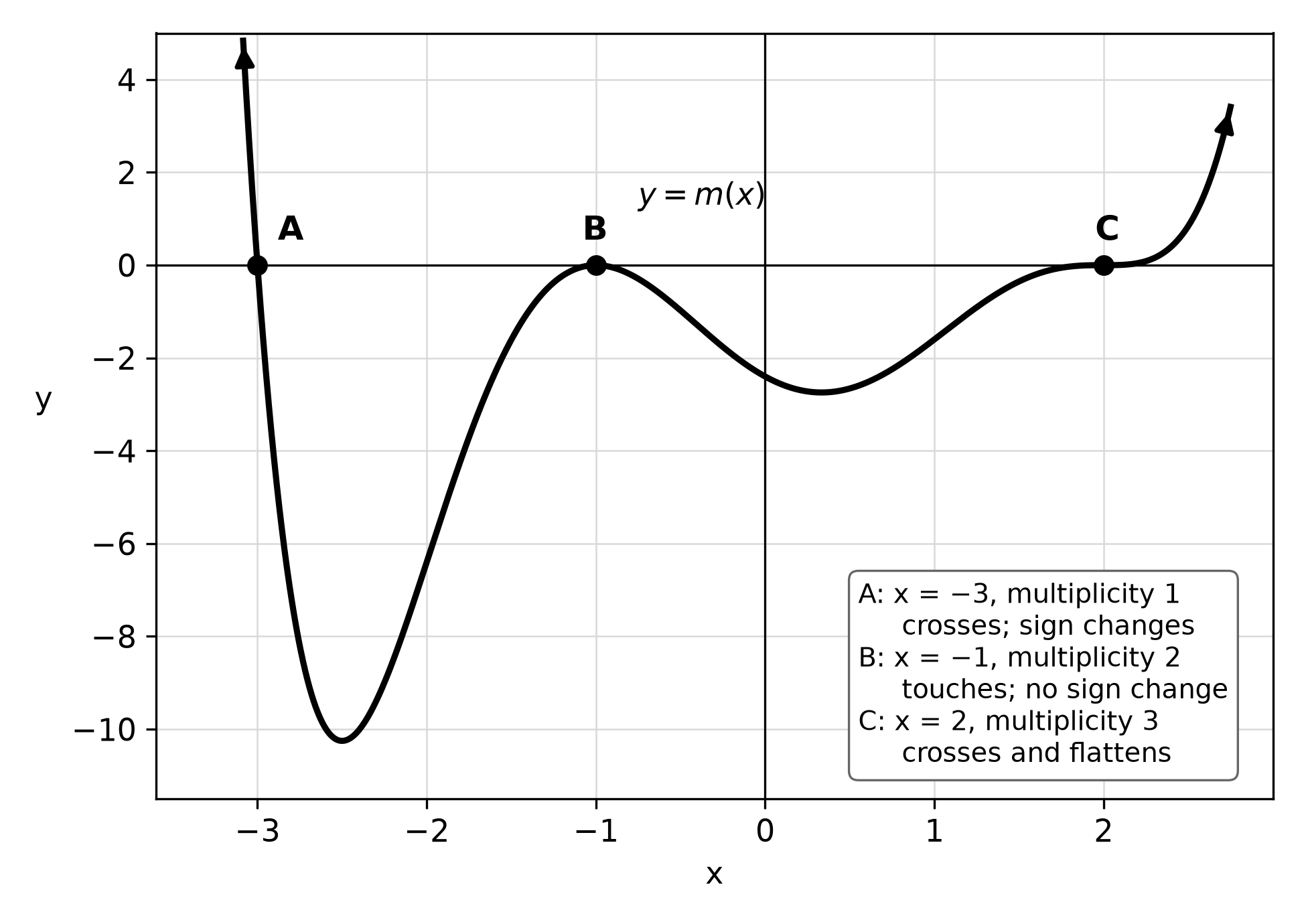
Figure 4.2. One polynomial with zeros of multiplicity 1, 2 and 3. Only the even-multiplicity zero leaves the sign unchanged.
To solve or , mark the real zeros on a number line. They are the only places where the sign can change. Find the sign in each interval by testing one input or by counting negative factors, and skip the sign change at every even-multiplicity zero.
Worked example 4.3: solve a polynomial inequality
Solve for .
The zeros are , 1 (multiplicity 2) and 3. The leading term is , so is negative for large . Start at the right: negative for ; the sign changes at 3, so is positive on ; it does not change at 1, so stays positive on ; it changes at , so is negative for . Include the zeros, because the inequality allows equality. The solution is . Check: and .
Worked example 4.4: zeros that are not real
Find all zeros of . Group the terms: . The zeros are 3, and : one real zero and one conjugate pair, three in all for degree 3. The graph crosses the -axis once.
Now reverse the process. Build a degree-3 polynomial with real coefficients, leading coefficient 2 and zeros 4 and . Real coefficients force to be a zero too, and the pair multiplies to . So . Expand it yourself and confirm that and .
Find the degree from equal-interval differences
For equally spaced inputs, subtract consecutive outputs, then subtract consecutive differences, and so on. A linear function has constant first differences and a quadratic has constant second differences. In general, the degree is the least for which the $n$th differences are constant. When the inputs step by , that constant equals .
Worked example 4.5: a pattern that misleads
A polynomial has degree at most 5 (constructed practice data).
| 0 | 1 | 2 | 3 | |||
|---|---|---|---|---|---|---|
| 2 | 2 | 2 | 47 |
First differences: , 3, , 3, 45. Second: 6, , 6, 42. Third: , 12, 36. Fourth: 24, 24. The fourth differences are constant, so has degree 4, and gives . The alternating outputs suggest a repeating pattern, but only the first constant row decides the degree.
Even and odd polynomials
A function is even if for every in its domain; its graph is symmetric about the -axis. It is odd if ; its graph is symmetric about the origin. A polynomial is even exactly when every term has an even power (a constant counts as ), and odd exactly when every term has an odd power. Mixed powers give a function that is neither. An odd polynomial must satisfy , so a nonzero constant term rules oddness out. Degree alone does not decide: has odd degree, yet its expansion contains and 8, so it is neither.
Try it 4.2. Classify , and as even, odd or neither.
End behavior from the leading term
The statement means the outputs increase without bound as the inputs increase without bound; the other three cases read the same way. For inputs of large magnitude, the leading term dominates every other term, so the degree and the sign of decide the ends.
| Degree | Leading coefficient | ||
|---|---|---|---|
| even | positive | ||
| even | negative | ||
| odd | positive | ||
| odd | negative |
The constant term and the middle terms play no part in end behavior.
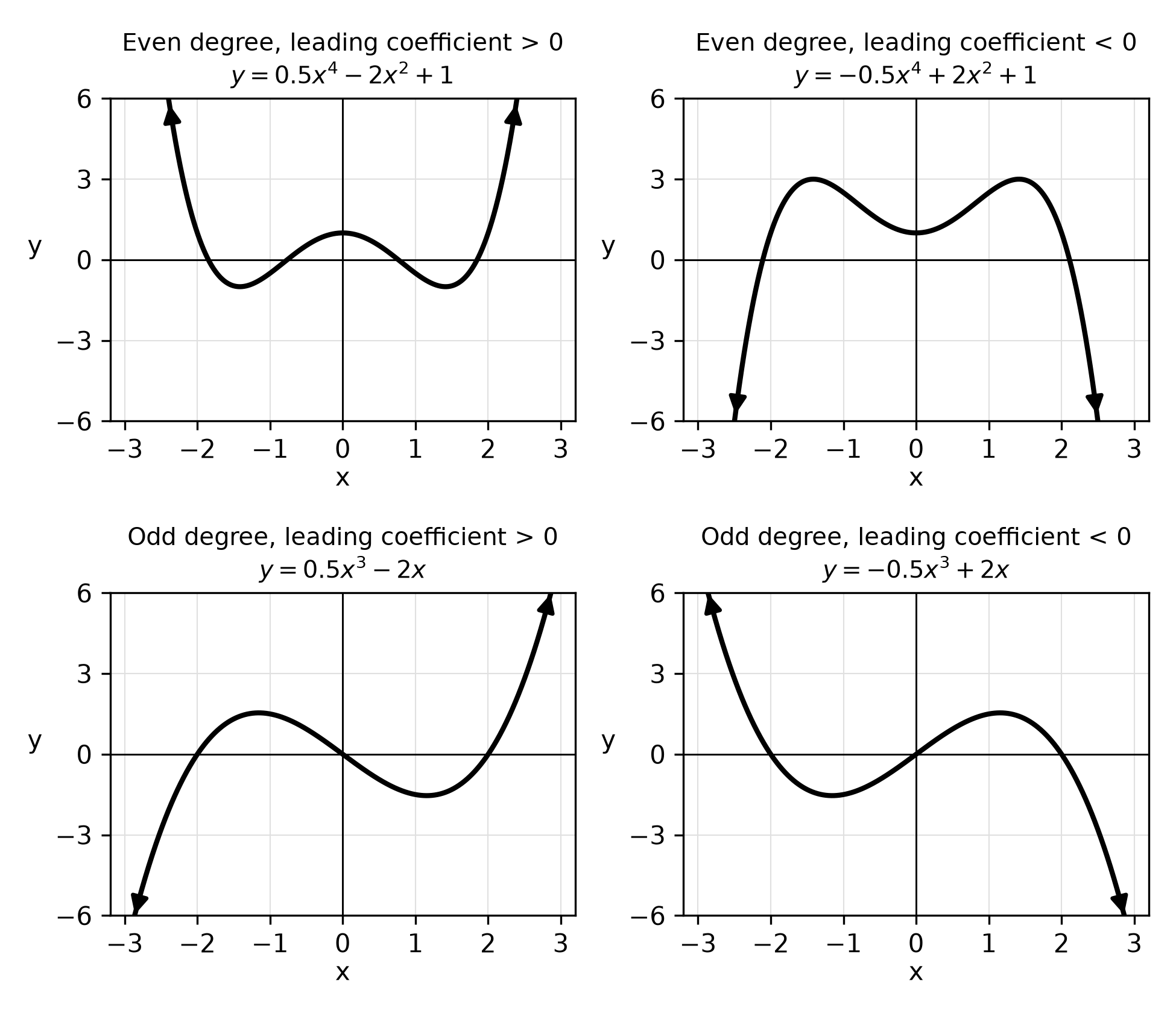
Figure 4.3. The four end-behavior patterns. The ends depend only on whether the degree is even or odd and on the sign of the leading coefficient.
A viewing window can mislead. In the window , the graph of seems to fall on the right, because . Yet ; the leading term eventually wins. Decide end behavior from the leading term, then choose a window that confirms it.
Worked example 4.6: end behavior from factored form
Describe the end behavior of .
Multiply the leading parts: . The degree is even and the leading coefficient is negative, so and . Check: and . If models a quantity only for , its end behavior describes the formula, not the situation, because the model's domain excludes both ends.
Try it 4.3. Describe the end behavior of and of with limit notation.
Use technology with a reason
On calculator questions, a graphing calculator finds zeros that do not factor, locates turning points and solves inequalities. Use it with three habits.
- Restricted domains. Built-in maximum and minimum features report turning points. Evaluate the included endpoints yourself.
- Apparent tangency. A graph that seems to touch the axis may turn just above it or cross twice nearby. Check the output at the turning point: unless it is 0, the turning point is not a zero.
- Precision. Keep full calculator values while you work, and round final answers to three decimal places unless a question says otherwise.
Repair common errors
| Error | Repair |
|---|---|
| Checking only turning points for a global extremum | Evaluate every included endpoint too. |
| Taking the term written first as the leading term | Find the highest power. |
| Expecting a sign change at every zero | Even-multiplicity factors keep their sign. |
| Forgetting a conjugate zero | With real coefficients, nonreal zeros come in pairs. |
| Reading the degree from the number of table rows | Find the first row of constant differences. |
| Deciding end behavior from one window | Use the leading term. |
| Calling a polynomial odd because its degree is odd | Check the power of every term. |
Check your try-it work
- is a local maximum at an included endpoint, because decreases just to the right of 0; is a local minimum; is a local maximum at the other included endpoint. The global maximum is 18 and the global minimum is . If you listed only , reread Worked example 4.1.
- is odd (powers 5 and 1), is even (powers 4, 2 and 0), and is neither (powers 3 and 2).
- For , the leading term is , so and . For , the leading term is , so both limits are .
Retrieve and review
Close the book and write, from memory, the four end-behavior cases and the rule linking multiplicity to crossing or touching. Then, without a calculator, solve and test one input in each interval. (The solution is ; the squared factor is never negative, and at the product equals 0, which a strict inequality excludes.) Tomorrow, rework Worked example 4.3 with the inequality reversed. In a week, sketch a degree-4 polynomial with a double zero and two nonreal zeros from its structure alone. Chapter 5 extends multiplicity to holes and vertical asymptotes of rational functions.
Practice
Twenty-two multiple-choice questions, Questions 51–72, and one free-response task, Written task 2, are printed after this chapter. Questions 57, 64, 65 and 72 require a graphing calculator; answer the other eighteen without one. Written task 2 is a six-point function-concepts task that requires a graphing calculator and has two pages of response space. Keys, the reasoning for every choice, the scoring guide and a complete sample response are under Chapter 4: answers and explanations in the answers section. Each explanation ends with a repair step that names the section of this chapter to revisit.