What to practice
- Distinguish zeros, holes and asymptotes; preserve restrictions through equivalent expressions.
Start with a graph that hides something
Graph in a standard calculator window and you will probably see two smooth branches separated by a vertical gap near . Nothing seems to happen at . Yet is undefined, exactly as is. Why does one excluded input produce a dramatic asymptote while the other removes a single point that many screens never show?
This chapter answers that question and the related ones the exam asks: where a rational function equals zero, where it is positive, how it behaves for inputs of large magnitude, and when two formulas define the same function. The central habit is easy to state and easy to abandon: record the domain of the original expression before you simplify it, and keep that record until the end. The chapter covers topics 1.7 to 1.11 of the AP Precalculus Course and Exam Description.
What a rational function measures
A rational function is a quotient of two polynomial functions, , where is not the zero polynomial. For each allowed input, compares the size of with the size of . That one interpretation explains almost every feature in this chapter. When is close to zero while is not, the quotient is huge. When is zero while is not, the quotient is zero. When both are zero at the same input, the quotient is undefined there, and you must look at nearby inputs to learn more.
The domain is every real number except the real zeros of the denominator. Write it first. For the opening example, , so the domain is all real with and .
The Fall 2026 clarification of the course framework states that two functions are equal only when they have the same domain and give the same output for every input in it (CED clarifications and corrections). Factoring and cancelling produce a simpler expression, but that expression usually has a larger natural domain. Treat it as a tool for studying the original function, not as a replacement for it.
End behavior comes from leading terms
For inputs of large magnitude, every polynomial is dominated by its leading term. A rational function's end behavior therefore follows the quotient of the leading terms of its numerator and denominator. Three cases result.
| Degree comparison | Quotient of leading terms | End behavior of the graph |
|---|---|---|
| Numerator degree smaller | constant over a nonconstant power | horizontal asymptote |
| Degrees equal | a nonzero constant | horizontal asymptote |
| Numerator degree larger | a nonconstant polynomial | follows that polynomial; slant asymptote when the degrees differ by one |
A horizontal asymptote means the outputs get arbitrarily close to and stay arbitrarily close as the inputs increase or decrease without bound. In limit notation, or . The asymptote describes far-away behavior only. It says nothing about inputs in the middle of the graph.
Worked example 5.1: three end behaviors
Describe the end behavior of , and .
For , the leading terms give , so and the horizontal asymptote is . For , the leading terms give , which approaches 0, so is the horizontal asymptote. For , the leading terms give . The graph of has no horizontal or slant asymptote; both ends rise like , so and .
Check. , close to 2 as predicted. When a function is given in factored form, multiply only the leading parts of the factors. In the leading terms are and , so the horizontal asymptote is . The constant terms, which give , play no part.
Worked example 5.2: a graph that meets its asymptote
Let . The denominator has discriminant , so it has no real zeros and the domain is all real numbers. Equal degrees give the horizontal asymptote .
Can the graph reach ? Solve . Because the denominator is never zero, multiplying by it is safe: , so and . The graph meets its horizontal asymptote at , rises above it, and then approaches 3 from above as increases (Figure 5.1a). A horizontal asymptote describes the ends of a graph; it is not a fence.
Worked example 5.3: find a slant asymptote by division
Let . The numerator's degree is one more than the denominator's, so expect a slant asymptote. Polynomial long division rewrites a dividend as divisor times quotient plus remainder, with the remainder's degree less than the divisor's. Divide by to get ; subtract to leave . Divide by to get 3; subtract to leave the remainder 5. So
and, for , . As grows, approaches 0, so the graph approaches the line . Check at : , the line gives 15, and the remainder term gives exactly . The leading-term quotient alone, , gives the correct slope but the wrong line; only the full division supplies the constant 3.
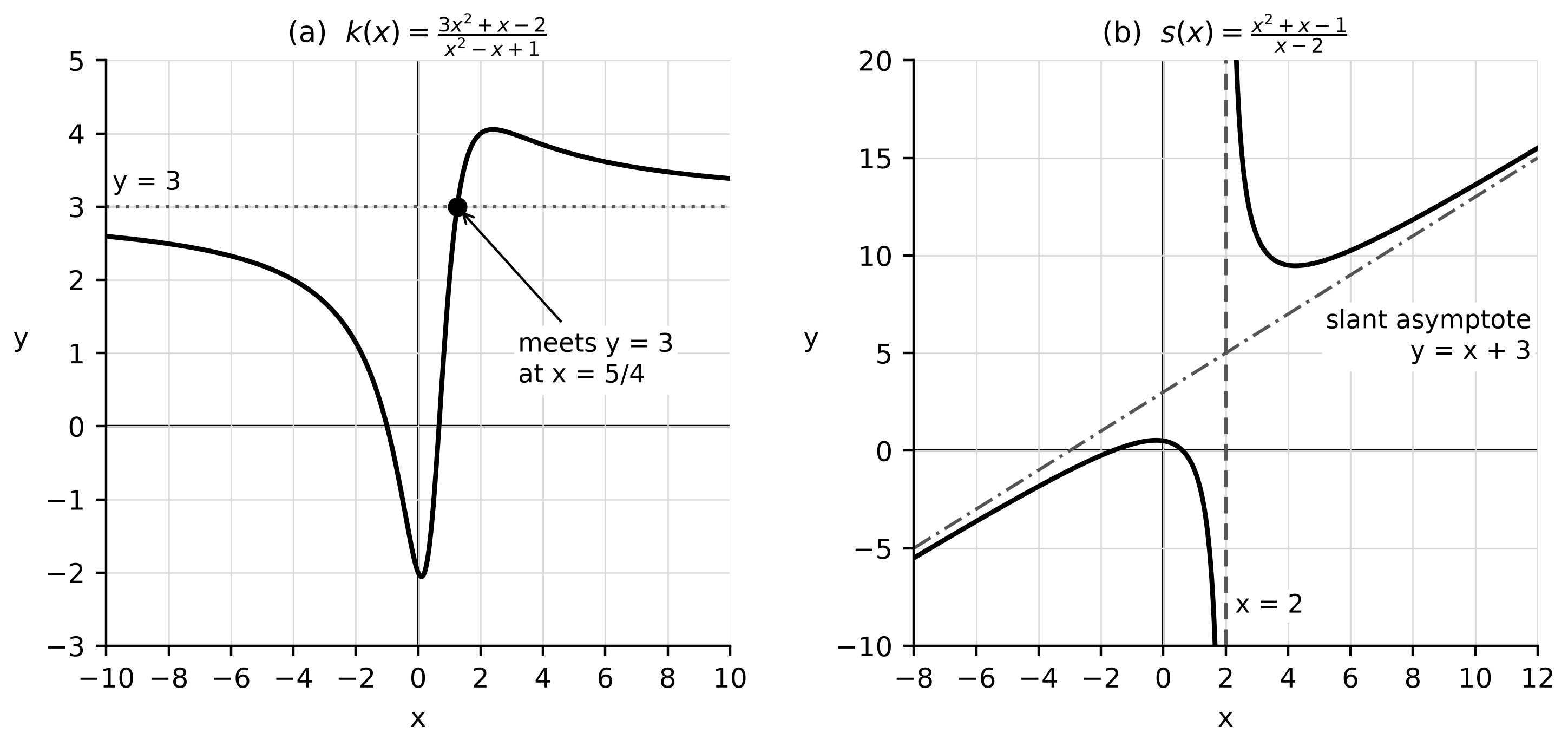
Figure 5.1. End behavior is about far inputs. (a) A graph can meet its horizontal asymptote and still approach it at both ends. (b) Long division gives the slant asymptote .
Zeros and sign changes
The real zeros of a rational function are the real zeros of its numerator that belong to its domain. Find the numerator's zeros, then test each against the original denominator. A numerator zero that also makes the original denominator zero is not a zero of the function; it is an excluded input, usually a hole.
To solve or , mark every real zero of the numerator and of the denominator on a number line. These are the only places where the sign of can change, because a quotient of polynomials changes sign only at a zero or at an excluded input. Test one input in each interval, or count negative factors. Numerator zeros are included when the inequality allows equality; denominator zeros are never included. A factor raised to an even power does not change sign.
Worked example 5.4: solve a rational inequality
Solve .
The boundary inputs are and 3 (numerator zeros) and 1 (denominator zero). Test , 0, 2 and 4: , , and . The sign does not change at 1 because is positive on both sides. Include and 3, where equals 0; exclude 1. The solution is (Figure 5.2).
Multiplying both sides of an inequality by a denominator is valid only when you know the denominator's sign. Here for , so multiplying gives , whose solution still needs 1 removed. For a denominator such as , whose sign changes at 1, the same shortcut produces wrong intervals.
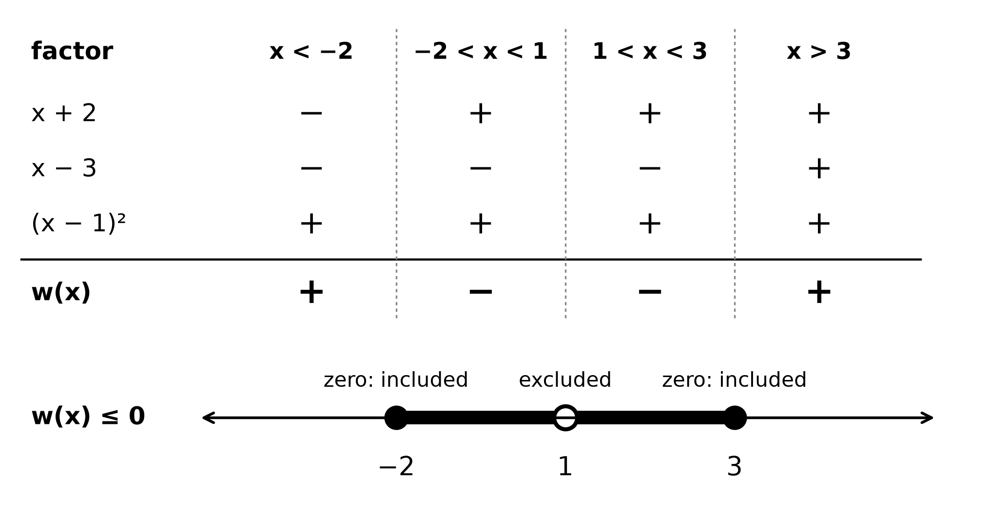
Figure 5.2. Sign chart for . The squared factor never changes sign, but the input 1 is still excluded.
Vertical asymptotes and holes: compare multiplicities
Every real zero of the original denominator is excluded from the domain, but excluded inputs produce two different graph features. Factor both polynomials completely and compare the multiplicity of each zero of the denominator.
- If has greater multiplicity in the denominator than in the numerator (including multiplicity 0 in the numerator), the graph has a vertical asymptote . Near the denominator is close to 0 while the reduced numerator is not, so the outputs increase or decrease without bound.
- If has multiplicity in the numerator greater than or equal to its multiplicity in the denominator, the graph has a hole at . The function is undefined there, but outputs for inputs near approach a single value , and the hole is the point .
Describe asymptote behavior with one-sided limits: uses inputs slightly greater than , and uses inputs slightly less. To find the sign, decide the sign of each factor for an input just to one side. At a hole, both one-sided limits equal , so , and you can compute by evaluating the reduced expression at .
Worked example 5.5: a hole and an asymptote in one function
Return to , with domain , .
At the factor appears once in each polynomial, so the multiplicities are equal: a hole. On the domain, , and at that reduced expression gives . The hole is . At the denominator factor has no match: a vertical asymptote. Just left of 2, ; just right, . So and . The zero is , which is in the domain, and the horizontal asymptote is . The two exclusions behave differently because only at does the denominator approach 0 while the numerator stays away from 0 (Figure 5.3).
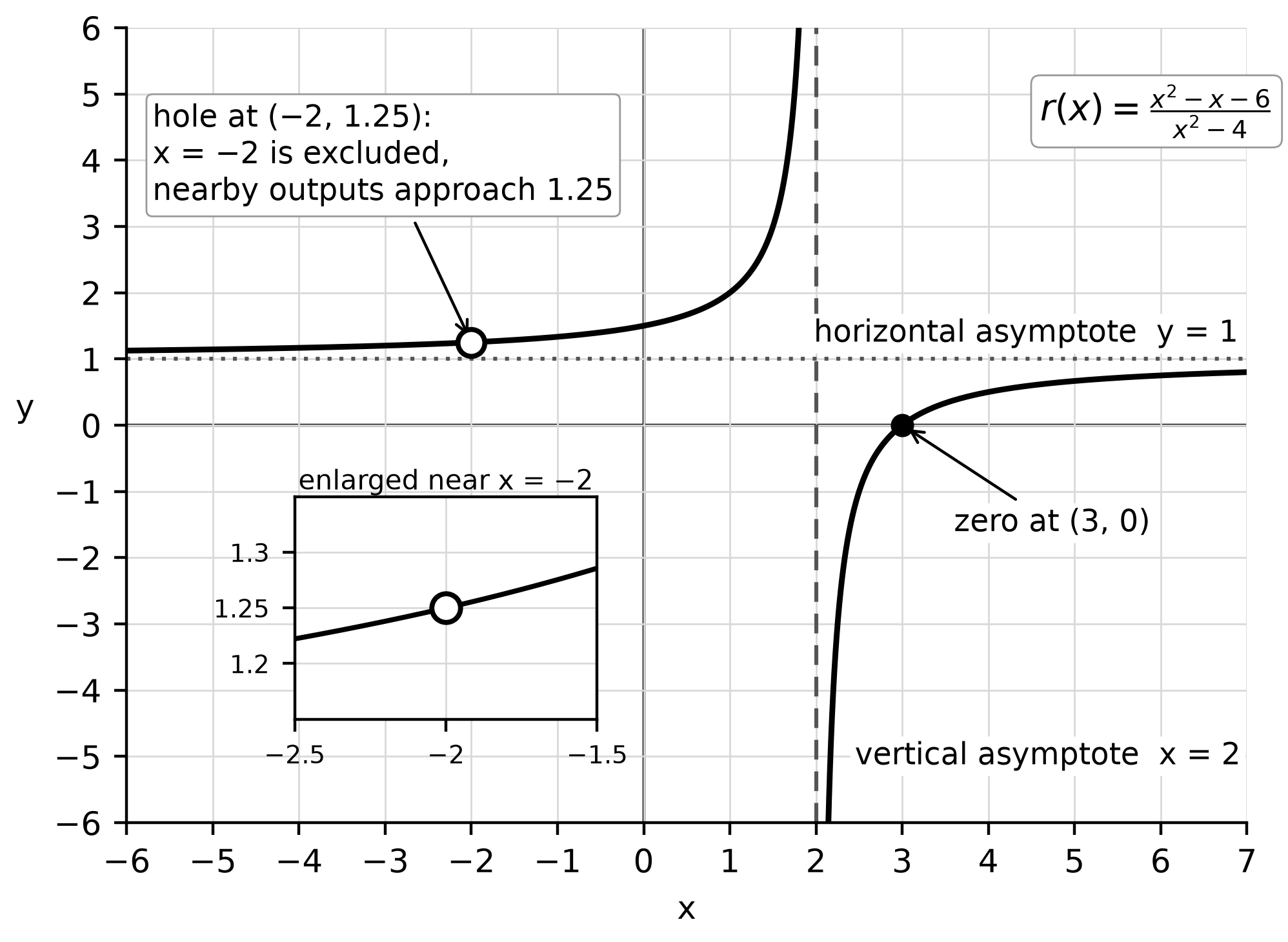
Figure 5.3. One function, two exclusions: a hole at and a vertical asymptote . The inset enlarges the missing point that a calculator screen can hide.
Worked example 5.6: a hole on the x-axis
Let , with domain , . At the numerator multiplicity 2 is greater than the denominator multiplicity 1, so the graph has a hole. On the domain, , which gives 0 at : the hole is . The missing point lies on the -axis, yet is not a zero of , because does not exist. At the denominator multiplicity 3 is greater than 1, so is a vertical asymptote. The remaining factor is squared and the reduced numerator is 3 there, so both one-sided limits are ; for example, and . This function has no zeros at all.
Equivalent forms with a purpose
Different equivalent forms answer different questions. Factored form reveals zeros, excluded inputs, holes, vertical asymptotes and sign changes. Standard form, or the quotient-plus-remainder form from long division, reveals end behavior. Choose the form for the question, and carry the original domain through every rewrite.
Worked example 5.7: equal expressions, unequal functions
Compare with . For every , . But is undefined while . The domains differ, so and are not equal functions; the graph of is the line with a hole at . A correct rewrite keeps the restriction: for .
Worked example 5.8: expand with the binomial theorem
The binomial theorem expands using one row of Pascal's triangle. Each row starts and ends with 1, and each interior entry is the sum of the two entries above it; row 4 is 1, 4, 6, 4, 1. The general term is , where is entry of row , counting from 0.
Expand with and :
The signs alternate because odd powers of are negative. Check at : and . The factored form shows a single zero at of multiplicity 4; the standard form shows the leading term and the -intercept 16.
Use technology without losing restrictions
On calculator sections, a graphing utility helps you find numerator zeros that do not factor, solve rational equations and inequalities numerically, and examine outputs near an excluded input. It cannot replace the domain record. A graph drawn from sampled points may not show a hole at all, and a table may give the same undefined message at a hole and at an asymptote. When a table reports no value at , evaluate inputs such as and . Outputs that agree and settle near one number indicate a hole; outputs that grow in magnitude indicate an asymptote. For the opening function, and , while and .
When you clear denominators to solve , the resulting polynomial equation is defined at the excluded inputs, so it can have solutions the original equation does not. Substitute every candidate into the original denominators and reject any that make one of them zero. A contextual model also has a domain set by the situation, such as nonnegative time or a tank's capacity; report only solutions inside it. Keep extra decimal places while you work, then round final answers to three decimal places unless told otherwise.
Common errors to repair
- Cancelling and forgetting. Simplifying to and then treating as allowed. Repair: write the domain before factoring and copy it beside every rewrite.
- Every excluded input is an asymptote. Repair: compare multiplicities; a shared factor whose numerator multiplicity is at least as large gives a hole.
- A cancelled numerator zero listed as an x-intercept. Repair: a zero must make the original function equal 0, so it must be in the domain.
- The asymptote as a fence. Repair: solve to see whether the graph meets its horizontal asymptote.
- Constant terms deciding end behavior. Repair: compare only leading terms; in factored form, multiply the leading parts.
- Brackets at denominator zeros. Repair: excluded inputs always get parentheses in a solution set.
- A sign change at every boundary. Repair: even-power factors keep their sign.
- The leading-term quotient as the slant asymptote. Repair: divide completely; the whole quotient polynomial is the asymptote.
Try it
Work these on paper before reading the solutions.
- For , state the domain, the zeros, any hole, the vertical asymptotes and the horizontal asymptote.
- Solve .
- Rewrite as a polynomial plus a fraction whose numerator has smaller degree than its denominator. State the slant asymptote and find where the graph meets it.
- Find the coefficient of in the expansion of .
- Write a rational function with a zero at , a hole at , a vertical asymptote and a horizontal asymptote . Give the hole's coordinates.
Check your try-it work
- , so the domain is , . On it, . Zero: . Hole: . Vertical asymptote: . Horizontal asymptote: . If you listed 3 as a zero, reread the section on zeros.
- Factor: . The boundaries are , , 0 and 3, and the signs from left to right are , , , , . The solution is , with brackets at the numerator zeros and parentheses at the excluded inputs.
- , so the expression equals . The slant asymptote is . The graph meets it where the remainder is 0: , so at . Check: . The denominator is never zero, so there is no vertical asymptote.
- The term is . The coefficient is 54, not 6.
- One answer is . At , the reduced form gives , so the hole is . Other correct answers exist, such as using in both polynomials; check that the leading-term quotient is 2.
Review and retrieval
Close the book and write, from memory, the rule that separates a hole from a vertical asymptote and the three end-behavior cases. Then explain in two sentences why and are different functions. Tomorrow, without notes, invent a function with one hole and one vertical asymptote, analyze it as in Try it 1, and check your hole with a table near the excluded input. In about a week, solve the worked inequality again with the inequality sign reversed. Chapter 4's multiplicity ideas support this chapter; Chapter 6 transforms these graphs; and Chapters 10, 12 and 16 reuse the same domain habit for compositions, logarithmic equations and trigonometric identities.
Practice
Twenty-four multiple-choice questions, Questions 73–96, and one free-response task, Written task 3, are printed after this chapter. Answer Questions 73–91, the first nineteen, without a calculator. Questions 92–96 and Written task 3 require a graphing calculator, and each of their stems says so; Written task 3 is a six-point function-concepts task with two pages of response space. Work under timed conditions before checking. Keys, the reasoning for every choice, the scoring guide and a complete sample response are under Chapter 5: answers and explanations in the answers section. Each explanation ends with a repair step that names the section of this chapter to revisit.