What to practice
- Track point transformations, select a model family, state assumptions and interpret parameters.
A model is a function chosen for a purpose. Before you trust one, you should be able to say how its graph was built from a simpler graph, why its function family fits the situation, and which inputs it can honestly be used for. The three sections of this chapter build those abilities in order: transformations as precise operations on inputs and outputs (topic 1.12), choosing a family from evidence (1.13), and building and applying a model on a defensible domain (1.14).
Quick prerequisite check. If , what is , and which input makes ? If you answered 5 and 1, you already have the two moves this chapter relies on: change an output after the function acts, and solve for the input that the original function must receive. If either answer felt uncertain, review function notation in Chapter 3 first.
Transformations act on inputs or on outputs
Every transformation in this course changes either the input before acts or the output after acts. Read an expression from the inside out and ask which of the two is being changed.
| Expression | What changes | Effect on the graph of |
|---|---|---|
| output | vertical translation by units (up when ) | |
| input | horizontal translation by units (left when ) | |
| output | vertical dilation by the factor when ; when , dilation by plus a reflection over the -axis | |
| input | horizontal dilation by the factor when ; when , dilation by plus a reflection over the -axis |
Output changes behave as written. Input changes feel backward because they happen before sees the input. In , the graph reaches the old input 0 when , so every feature arrives five units earlier, which means five units to the left. In , the old input 6 is reached when , so the graph is squeezed toward the -axis by the factor .
Transformations also change the domain and range. Input changes move or stretch the domain; output changes move or stretch the range. A reflection reverses the order of the endpoints it touches, so always recheck which endpoint is now smaller.
A reliable method: solve for the new input
Slogans such as "inside does the opposite" break down on combined transformations. Use equations instead. Suppose is on the graph of and
First, the input of must equal , so solve for . Second, the output of at that moment is , so the new output is . The point therefore moves to . The same two equations transform domain endpoints and range values, so one method answers every question about a transformed graph.
Worked example 6.1: transform a point, a domain and a range
The function in Figure 6.1 is defined for , passes through , , and , and has range . Let .
Point. For , solve , so . The new output is . The image is .
Domain. The input of must stay between 0 and 4, so , which gives .
Range. Multiply the extreme outputs by first: becomes and becomes , so the order reverses. Then add 1. The range of is .
Check. In Figure 6.1 the solid graph runs from to , its lowest points are and at height , and its highest point is , matching all three results.
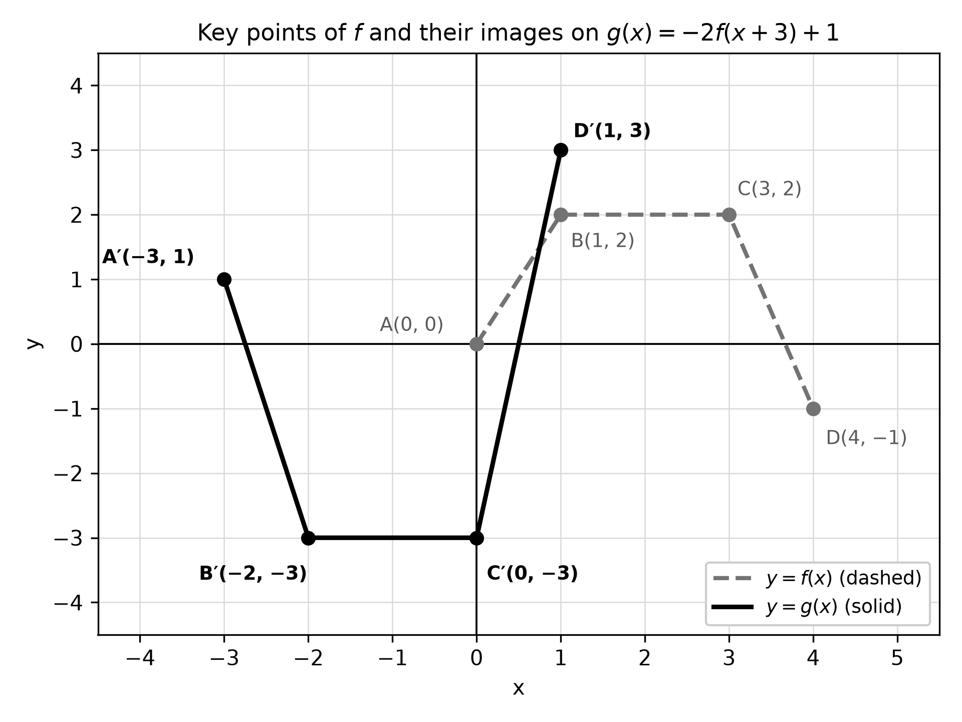
Figure 6.1. Each labeled point of and its image on . The letters let you check each pair.
Worked example 6.2: factor before you read a horizontal shift
Describe as a sequence of transformations. Apply the method to a general point : solving gives . Every input is halved and then increased by 3, so the graph undergoes a horizontal dilation by the factor followed by a translation 3 units right. Factoring shows the same fact: .
A second order is also correct: translate 6 units right, giving , then dilate horizontally by , giving . The common error mixes the two descriptions, dilating first and then translating 6 units. That produces , a different function. Test any description with one point: for on , the correct image has , and confirms it.
Errors to catch before they cost points
- Moving in the wrong horizontal direction: with moves left.
- Using instead of as the horizontal dilation factor.
- Adding before multiplying on the output side. In the output of is multiplied by first.
- Forgetting that a negative factor reverses the order of the endpoints of a range or domain.
Try it 6.1. The function has domain , range , and lies on its graph. Let . Find the image of , the domain of and the range of .
Check your work. Solve to get ; the new output is , so the image is . For the domain, gives ; the reflection reversed the endpoints. For the range, and , so the range is . The positive factor keeps the range endpoints in order.
Choose a model family for a reason
A function family is a promise about how outputs change. Choose the family whose promise matches the evidence, state the assumption you are making, and name what would break the promise.
| Evidence over equal input steps or from the context | Family it supports |
|---|---|
| constant first differences (equal output changes) | linear |
| constant second differences; one turning point; symmetry about a vertical line | quadratic |
| constant third differences; a volume built from three lengths that each depend on | cubic |
| a fixed total shared among parts; outputs that level off toward a value | rational |
| different rules on different input intervals, such as a rate that changes at a threshold | piecewise |
Two cautions apply. Differences reveal a family only when the inputs are equally spaced; with unequal spacing, compare average rates of change instead. And a pattern in a few points is evidence, not proof. Real measurements are rarely exact, so look for differences that are approximately constant, then ask whether the context gives a reason for the pattern: an area built from two growing lengths suggests a quadratic, and a fixed job split among workers suggests a rational model.
Worked example 6.3: select a family from constructed data
The table gives constructed practice data for the braking distance of a test cart.
| Initial speed (m/s) | 2 | 4 | 6 | 8 | 10 |
|---|---|---|---|---|---|
| Braking distance (m) | 1.6 | 5.2 | 10.8 | 18.4 | 28.0 |
The speeds are equally spaced, so differences are meaningful. The first differences are 3.6, 5.6, 7.6 and 9.6, so a linear model is ruled out. The second differences are 2.0, 2.0 and 2.0, which supports a quadratic model. The quadratic reproduces every value; for example, .
Figure 6.2 shows why the linear regression line is a poor choice even though it rises with the data. It lies above the middle points and below the end points, a curved pattern of misses that no line can remove. It also predicts a negative braking distance for speeds below about 2.1 m/s, which is impossible.
Assumption. The cart, surface and braking force stay the same at every tested speed. What would contradict the model: second differences that drift steadily, or a new trial whose distance lies far from the curve.
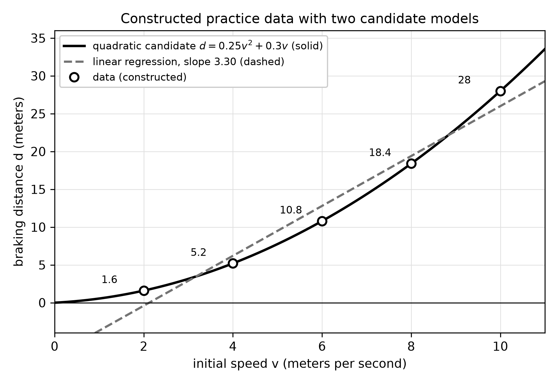
Figure 6.2. Constructed practice data with a quadratic candidate and a linear regression line. The line's misses are systematic, not random.
Worked example 6.4: choose a family from the context alone
A town plans 600 volunteer-hours to clear a riverbank, shared equally among volunteers. Each person's hours satisfy , so . Doubling the volunteers halves each share, the signature of inverse proportion and therefore a rational model. A linear rule such as would eventually give zero or negative hours, which the context forbids. The contextual domain is the positive whole numbers; the rational expression is undefined at , where its vertical asymptote lies.
Errors in choosing a family
- Computing differences across unequal input steps.
- Calling every increasing pattern linear.
- Accepting a model because its graph looks right in one viewing window.
- Treating a close fit as proof that the pattern continues beyond the data.
Try it 6.2. Constructed data: for the outputs are 2, 9, 28, 65 and 126. Which polynomial family fits, and what evidence supports it?
Check your work. The first differences are 7, 19, 37 and 61; the second differences are 12, 18 and 24; the third differences are 6 and 6. Constant third differences support a cubic model, and matches every value. A complete answer also names one check outside the table, such as a new observation at , where the cubic predicts 217.
Build the model, then use it honestly
There are three common ways to construct a model. From conditions: pick a form whose parameters match what you know, such as vertex form for a known highest point, factored form for known zeros, or for inverse proportion, then use one more condition to find the remaining parameter. From data with technology: enter the data as lists, choose the regression family you justified, and keep the unrounded coefficients for every later calculation. Piecewise: build each piece separately, state each piece's input interval, and check the values where the pieces meet.
Then apply the model: evaluate it, solve with it, interpret each parameter with units, and state the contextual domain, which is the set of inputs for which the model's assumptions plausibly hold. The contextual domain is usually much smaller than the algebraic domain.
Worked example 6.5: construct a quadratic from conditions
A fountain jet leaves its nozzle at ground level, reaches its highest point 3 m above the ground at a horizontal distance of 4 m, and lands 8 m from the nozzle. Model the height , in meters, at horizontal distance .
The highest point suggests vertex form: . The nozzle condition gives , so and . Check the landing point: . The contextual domain is and the range is ; outside that interval the formula describes no water at all.
Will the jet clear a sculpture 2.4 m tall standing 2 m from the nozzle? Evaluate . Because , the jet hits the sculpture about 0.15 m below its top, as Figure 6.3 shows. The parameter means the jet drops m below its peak height at 1 m on either side of the peak, and four times as much at 2 m.
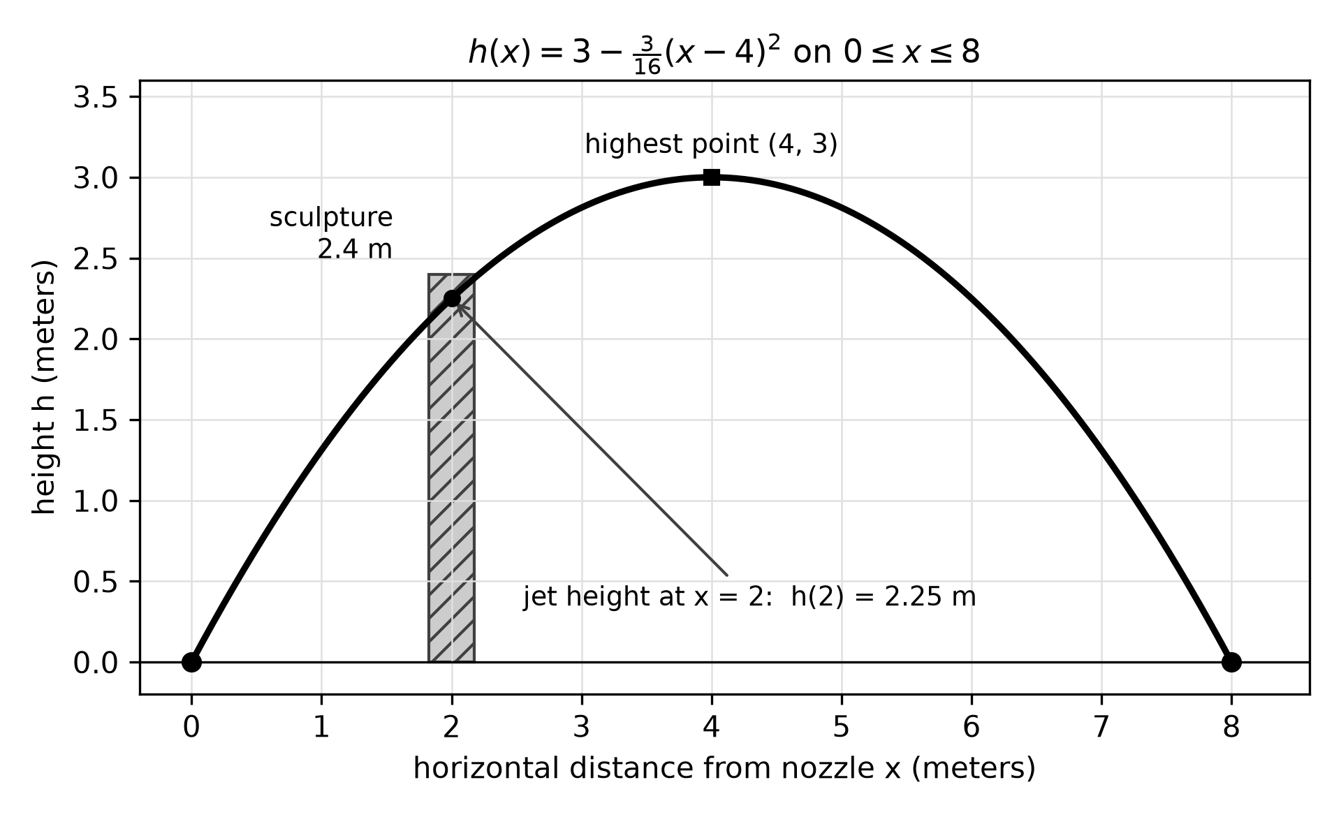
Figure 6.3. The model built from three conditions, checked against an obstacle. A model answers a design question only after it is evaluated at the relevant input.
Worked example 6.6: regression, then a decision (calculator)
Constructed practice data for a school play show tickets sold at five trial prices , in dollars: 6, 8, 10, 12 and 14 dollars gave 412, 371, 318, 279 and 236 tickets. The organizers want the price that maximizes predicted revenue.
The changes in over equal price steps are , , and , roughly constant, so a linear demand model is reasonable. Linear regression gives . The slope means that each 1-dollar increase in price predicts about 22.2 fewer tickets sold. Revenue is price times tickets, so , a quadratic built from the regression. Graphing and locating its maximum gives dollars, with predicted revenue of about 3,347 dollars.
Now judge the result. The maximizing price lies inside the tested prices from 6 to 14 dollars, so it is an interpolation. The model would predict zero tickets at about 24.56 dollars and negative sales beyond, so it must not be used far outside the observed prices. A sensible recommendation is a price near 12 dollars, checked against actual sales.
Errors in building and applying models
- Rounding regression coefficients before using them; small rounding errors grow when the model is evaluated far from the origin.
- Interpreting a parameter without its units or its input interval.
- Reporting a solution that lies outside the contextual domain.
- Evaluating the wrong piece of a piecewise model.
Try it 6.3. A courier charges 9 dollars for any parcel up to 2 kg. For kilograms the charge is dollars. Find the charge for a 7.2 kg parcel, the weight of a parcel that costs 36.50 dollars, and explain what the model says about a 25 kg parcel.
Check your work. Because , use the second piece: dollars. For 36.50 dollars, , so kg, which lies in the second piece's interval. A 25 kg parcel is outside the model's domain, so the model gives no charge for it; using the formula anyway would be an unsupported extrapolation.
Common errors to repair
| Error | Repair |
|---|---|
| Wrong shift direction, or used for | Worked examples 6.1 and 6.2 |
| Differences taken across unequal steps | Worked example 6.3 |
| Rounded coefficients; answers outside the contextual domain | Worked examples 6.5 and 6.6 |
Review and retrieval
Answer these from memory, then check against the chapter.
- Write the image of under and explain each coordinate.
- Give the evidence that supports each of the five families in the model-selection table.
- Explain the difference between an algebraic domain and a contextual domain, using the fountain jet.
- State one assumption behind any model you built in this chapter and one observation that would contradict it.
At your next study session, redo Try it 6.1 on blank paper. About a week later, invent a function on a closed interval, apply a transformation with a reflection, and predict its new domain and range before graphing. Chapter 9 extends model choice to exponential regression and residuals.
Practice
Twenty multiple-choice questions (Questions 97–116) and then two free-response tasks (Written tasks 4–5) follow this chapter. Work Questions 97–109 by hand. Questions 110–116 and both free-response tasks require a graphing calculator; keep unrounded values until your final answer. Each free-response task has two response pages and six points. Answer all items before checking. Keys, reasoning for every choice, repair directions and scoring guides with sample responses are under Chapter 6: answers and explanations.