What to practice
- Construct exponential models, compare alternatives, inspect residuals and bound extrapolation.
Chapter 8 started with a formula and asked what it says. This chapter runs the other way. You start with conditions or data, build an exponential model, and then test whether the model deserves to be used. A model is a claim about how a quantity behaves. It earns trust when its parameters have a clear meaning, its predictions stay inside the situation it describes, and its errors show no pattern.
Every data set in this chapter is constructed practice data created for this book. Values are given to enough decimal places for you to reproduce each regression on a graphing calculator.
Build a model from conditions
An exponential model has two parameters, so two pieces of information are enough to determine it. The information can be an initial value and a growth or decay rate, two input-output pairs, or one input-output pair and a rate. If two outputs come from inputs that are units apart, their ratio equals . Solve for the base first, then for .
A second form avoids computing at all. If the model passes through , then
This point-ratio form reads directly: start from a known output and apply the factor once for each unit of input beyond . It works the same way that point-slope form works for a line.
Worked example 9.1: two observations, neither at zero
A constructed model for the number of members of a reading forum, in hundreds, satisfies and , where is months after launch. Find and predict .
- Use the ratio. The inputs are 3 units apart, so .
- Solve for the base. , because .
- Solve for . , so .
- Predict. , about 9,113 members.
The value is the model's output at . It is not an observation, because no data were recorded at launch. Writing "the forum had 800 members at launch" overstates what the data show.
Worked example 9.2: point-ratio form
A constructed model for a laboratory culture, in thousands of cells, satisfies and , where is hours after the culture is started.
The two-hour ratio is , so and . In point-ratio form, . To compare with general form, , so . Both forms give : the first as and the second as . The point-ratio form is often faster and keeps the arithmetic close to the data.
Transformations, percent change and the natural base
An exponential model can be stretched, reflected and shifted like any function. A vertical shift is the transformation most often hidden in data. When a quantity levels off toward a value instead of toward 0, the differences may be proportional even though the outputs are not. Model the differences, then add back: .
A percent change gives the base. Growth of percent per unit gives , and decay of percent per unit gives . A 4% decrease per day is a factor of 0.96 per day.
Some models use the natural base . A model written as is still an exponential function in general form, because . The base for one unit of input is , not . For example, has the one-unit factor , an increase of about 5.13% per unit of , slightly more than 5%.
Worked example 9.3: growth with a ceiling
A constructed model for the height of a hedge, in centimeters, years after planting is
The heights at are 30, 60, 84 and 103.2 cm. They increase, yet the base is less than 1. The reason is : the expression shrinks, and subtracting a shrinking amount from 180 leaves a growing height. The distances below 180 are 150, 120, 96 and 76.8 cm, each 80% of the one before. The model predicts that the hedge approaches 180 cm but never passes it, which is a reasonable claim for a trimmed hedge with a planned height.
Use a model within its contextual domain
A model's domain in context is not all real numbers. It is the set of inputs for which the situation, the data and the model's assumptions all make sense. Times before a process began, counts larger than the population that could be counted, and inputs far outside the observed data all fall outside it. A prediction inside the observed inputs is an interpolation. A prediction beyond them is an extrapolation, and its reliability depends on whether the pattern continues, which the data cannot confirm.
Worked example 9.4: how far beyond the data?
Use from Worked example 9.2 to estimate when the culture reaches 1,000 thousand cells. A graphing calculator gives the intersection of and at hours.
Report the result with its limits. The observations ran only from hour 3 to hour 5. A value such as is a modest extrapolation. The estimate of 8.5 hours lies more than three hours beyond the data and assumes 50% hourly growth continues the whole time. Cultures run short of space and nutrients, so a careful answer reads: "If growth continued at the observed rate, the culture would reach about one million cells after about 8.5 hours; the data do not show whether growth continues that long."
Compare competing models
Before running a regression, look at the data as Chapters 6 and 8 showed.
- Roughly equal differences over equal input steps suggest a linear model.
- Roughly equal second differences, or a single change from increasing to decreasing, suggest a quadratic model.
- Roughly equal ratios over equal input steps, with outputs of one sign, suggest an exponential model.
A graphing calculator then finds the parameters. Linear and quadratic regressions use least squares. Exponential regression is more subtle. In Desmos, the default fit chooses and to minimize the squared differences between the data and the model's outputs. Desmos's optional log mode, and the ExpReg command on TI calculators, instead fit a line to the logarithms of the outputs. The two methods usually give slightly different values. This book's practice items accept either method and give a tolerance for each answer.
The constructed data in Figure 9.1 record a new subscription service's registered users, in hundreds, weeks after launch.
| Week | 0 | 1 | 2 | 3 | 4 | 5 | 6 | 7 |
|---|---|---|---|---|---|---|---|---|
| Users (hundreds) | 3.2 | 4.4 | 5.9 | 7.6 | 10.7 | 14.7 | 19.7 | 26.4 |
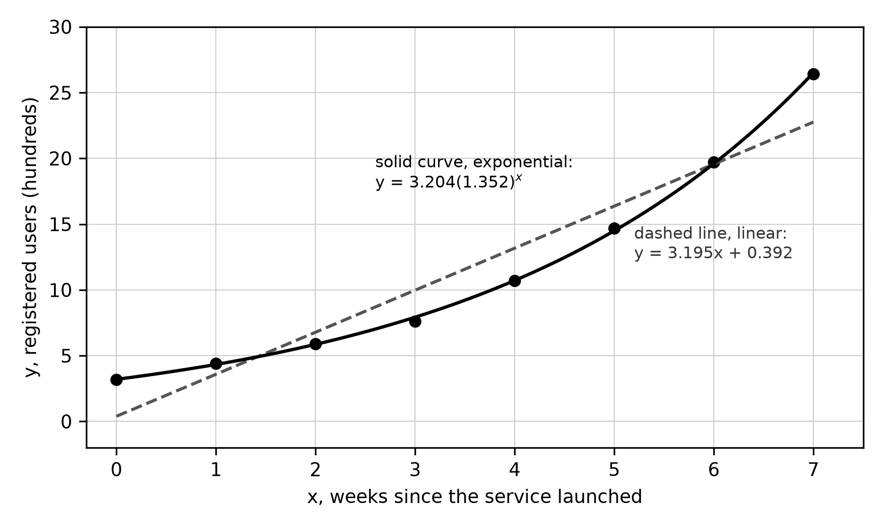
Figure 9.1. Constructed practice data with two regressions. The curve follows the points closely; the line misses them in a systematic way. Original graph.
Validate with residuals
A residual measures how far an observation lies from a model's prediction:
A positive residual means the model underestimates that observation. A negative residual means it overestimates. Both kinds are errors, so a signed residual shows direction, while its absolute value shows size.
A residual plot graphs each residual against the independent variable. If the points scatter above and below 0 with no clear pattern, the model is appropriate for the data. If they form a pattern, such as positive at both ends and negative in the middle, the model misses a systematic feature of the data and another model should be considered. Small residuals alone are not enough, and neither is an equal count of positive and negative residuals. The pattern is what matters.
Context can also decide which error is safer. A model that sets how much road salt to order should not underestimate need, so a planner might prefer a model whose errors tend to be overestimates. A model that schedules staff to match demand might be preferred if it seldom overestimates. That preference matters only after a model passes the residual-pattern test.
Worked example 9.5: residuals by hand
A constructed model is . The observed values at are 2.1, 3.8, 8.3 and 15.9. The predictions are 2, 4, 8 and 16, so the residuals are , , and . At the model overestimates by 0.2. The signs alternate without a trend and the sizes stay small relative to the outputs, so these four points give no evidence against the model.
Worked example 9.6: choosing between two regressions
Use the registered-user data from Figure 9.1, with a graphing calculator.
- Fit both models. Linear regression gives . Exponential regression gives with the default method, or with logarithms.
- Compute residuals. For they are 2.808, 0.813, , , , , 0.137 and 3.642. For with the default method they are , 0.067, 0.040, , , 0.208, 0.101 and . The other exponential fit gives residuals with the same signs.
- Read the plots. In Figure 9.2A the linear residuals are positive at both ends and negative in the middle, a U shape. In Figure 9.2B the exponential residuals stay close to 0 and show no U shape. The panels use different vertical scales; the exponential residuals are also about ten times smaller.
- Decide and explain. The exponential model is more appropriate because its residual plot shows no pattern, while the linear residual plot curves.
- Predict with limits. At week 10 the models give about 32.3 hundred (linear) and 65.5 hundred (exponential: 65.55 by default, 65.46 with logarithms). The exponential prediction is better supported, but week 10 is three weeks past the data, so it is an extrapolation.
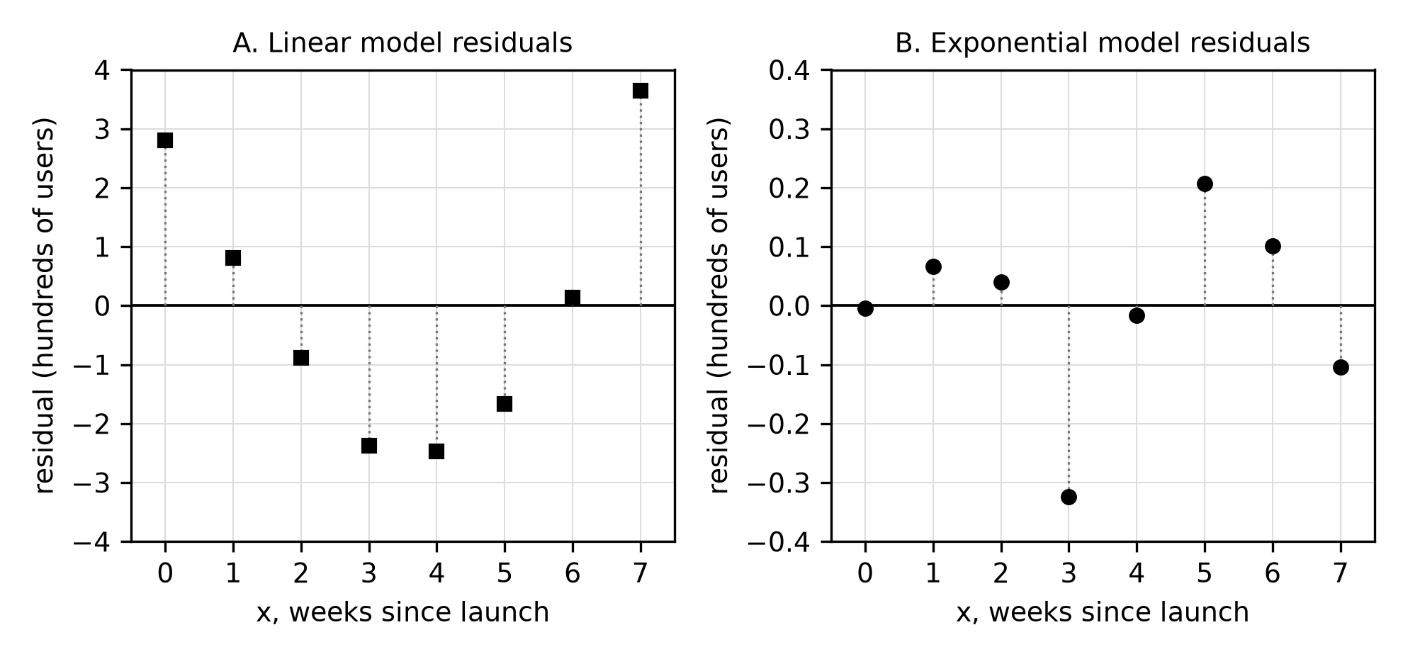
Figure 9.2. Residual plots for the two regressions in Worked example 9.6. Note the different vertical scales. Original graph of constructed practice data.
Errors to catch before they cost points
- Residual sign reversed. Residual means actual minus predicted. A positive residual is an underestimate.
- Initial value treated as data. If no observation was made at , then is a model value, not a measurement.
- Index mismatch. Enter the inputs the problem defines. Entering weeks 1 to 8 as 0 to 7 changes and every prediction.
- Small residuals taken as proof. A model can have small residuals and a clear pattern. Judge the plot.
- Exponential regression on leveling data. If outputs approach a value , fit , not .
- Prediction without a domain. State whether a prediction is inside the observed inputs, and do not report outputs the context cannot produce.
Guided attempt
A constructed model for a culture count, in thousands, is , where is days. The observed count on day 4 was 74.1 thousand.
- Predicted value: ______.
- Residual: actual minus predicted ______.
- Complete the sentence: the model ______ the day 4 count by about ______ cells.
Check your reasoning. , so the residual is thousand. The residual is positive, so the model underestimates the day 4 count by about 1,170 cells.
Independent check
A constructed model for the percent of a pond's surface covered by algae is , built from observations on days 2 through 10. With a calculator: (a) interpret 1.6 in context, (b) find the residual on day 6 if the observed coverage was 12.3%, and (c) decide whether the model should be used to predict coverage on day 14.
Model reasoning. (a) The model predicts 1.6% coverage on day 0, but day 0 lies outside the observed days, so the value is a model estimate rather than a measurement. (b) , so the residual is percentage points; the model underestimates. (c) , which is impossible for a percent of a surface. Day 14 lies outside the contextual domain, and the model must be restricted to inputs where its outputs stay at or below 100%.
Retrieval and review
Without notes, write the residual definition, the meaning of a positive residual, and the decision rule for a residual plot. At your next study session, reproduce Worked example 9.6 on your own calculator and record which exponential method it uses. A week later, explain in three sentences why a model with small residuals can still be inappropriate. Chapter 12 adds semi-log plots, which turn exponential patterns into straight lines.
Practice
Attempt the printed Chapter 9 practice set before reading any solution. It contains fourteen multiple-choice questions, Questions 141–154, followed by Written tasks 7–8. Several questions share a printed data table or residual plot; a note above each shared source names the questions that use it.
- No calculator: Questions 141–145.
- Graphing calculator required: Questions 146–154 and both written tasks. Report values correct to three decimal places unless a question says otherwise. Either exponential regression method is accepted within the stated tolerance.
Allow about 30 minutes for the multiple-choice questions and 15 minutes for each written task, then check your work in "Chapter 9: answers and explanations" in the answer section. For each miss, follow the repair note printed with the explanation, rework the named example, and retry a fresh question two or three days later.