What to practice
- Solve equations/inequalities, assess contextual solutions and read semi-log displays.
Unit 2 ends with three decisions that a calculator cannot make for you. When you solve an exponential or logarithmic equation, you decide which candidates the original statement actually allows. When you build a logarithmic model, you decide what the input and output measure and where the model makes sense. When you read a semi-log plot, you decide whether equal vertical spacing means equal differences or equal ratios. This chapter covers topics 2.13 to 2.15 of the AP Precalculus Course and Exam Description. Keep Chapter 11's rules in view: a logarithm needs a positive argument, and its base is positive and not 1.
Keep a restriction record before you solve
The inverse relationship lets you move between forms: means exactly the same as . Properties of exponents and logarithms let you combine terms. Some of those moves, however, change the set of allowed inputs. Rewriting as is valid only when and , yet the combined form also accepts inputs that make both factors negative. Rewriting as accepts negative values of . Use three steps every time:
- Record the restrictions from the original statement.
- Solve the transformed relation.
- Test every candidate in the original statement, not in the transformed one.
A candidate that satisfies the transformed relation but breaks a restriction is an extraneous solution. The framework also asks you to reject results that the context rules out, such as a negative time.
Worked example 12.1: reject a candidate that leaves the domain
Solve .
Restrictions. The arguments must be positive: and , so .
Transform. The product property gives , so . Then , which factors as . The candidates are 8 and .
Check in the original. For : . For , is undefined, so is rejected. The solution is only.
Figure 12.1 shows why. The left side exists only to the right of , and there its graph meets the line once. The candidate belongs to the polynomial equation, not to the original function.
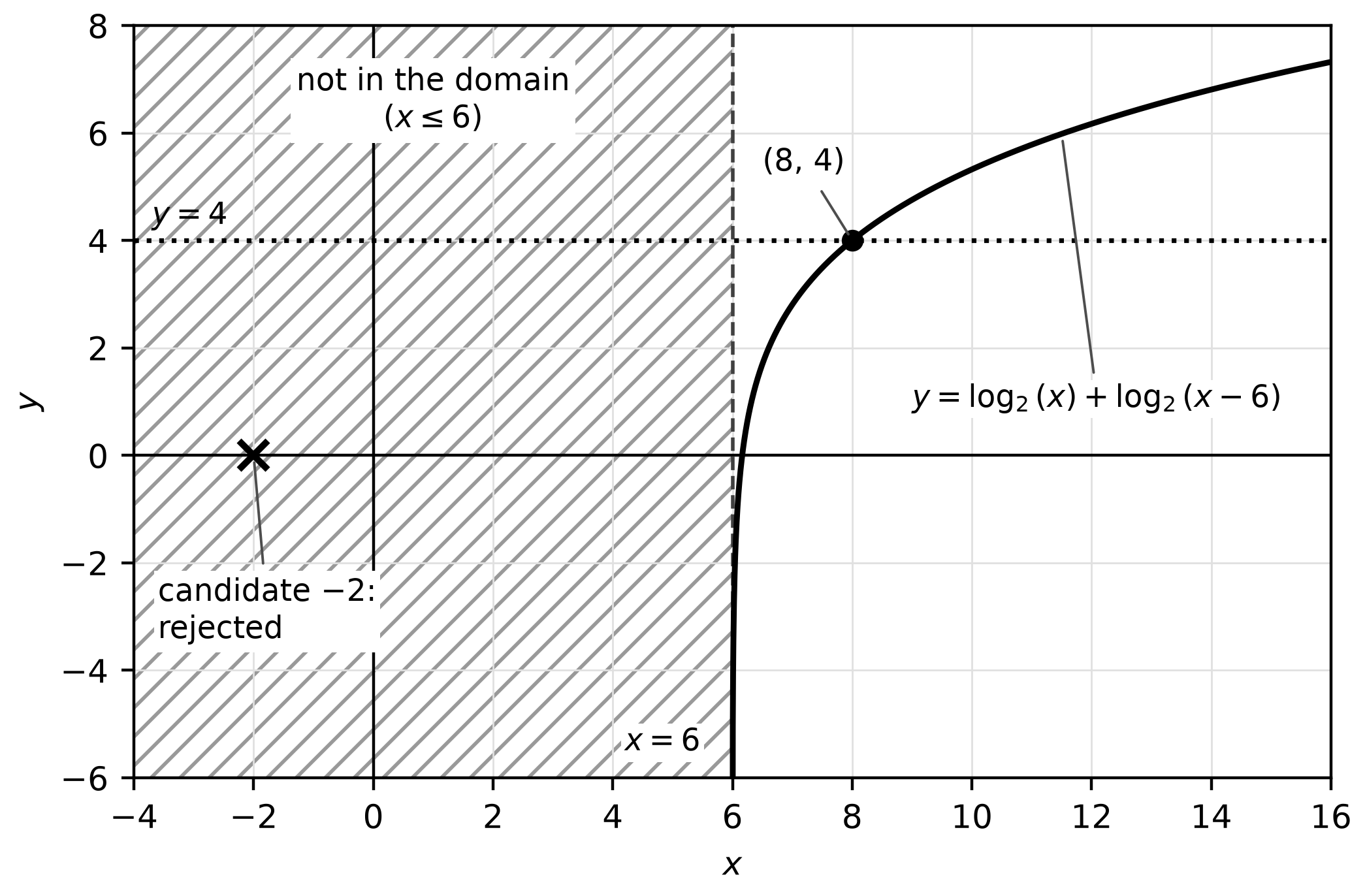
Figure 12.1. The original equation has one solution; the second candidate comes from the transformed polynomial and lies outside the domain.
Worked example 12.2: use logarithms when the bases differ
Solve exactly. Both sides are positive for every real , so the equation adds no restriction. Take the natural logarithm of both sides:
Collect the terms: , so
Check: both sides are approximately 11.974 at this value. Any base would work; the natural logarithm keeps the algebra tidy. The same idea rewrites an exponential in a new base, . For example, a quantity that doubles every 5 hours, , can also be written , so its continuous rate constant is per hour.
Inequalities follow the direction of the function
Exponential and logarithmic functions are one-to-one. Each is increasing when its base is greater than 1 and decreasing when its base is between 0 and 1. Applying an increasing function to both sides of an inequality keeps its direction; applying a decreasing function reverses it. Dividing by a negative number such as reverses it for the same reason.
Worked example 12.3: a decreasing base in a constructed context
A filter removes 20% of a contaminant on each pass, starting from 40 milligrams, so after passes. For which passes is ?
Divide by 40: . Take natural logarithms: . Because , dividing reverses the inequality: . Passes are whole numbers, so the amount is below 10 milligrams from the 7th pass on. Check: and .
A logarithmic inequality also carries its domain. For , the argument requires , and because is increasing, . Together, . Writing only includes inputs where the logarithm is undefined.
Try it 12.1 (partly done). Solve . The restriction is . The quotient property gives . Finish the solution and check it.
Check your work. The fraction equals , so and . Since , test it: .
Undo the mapping to build an inverse
Functions such as and are transformations of the basic exponential and logarithmic functions. To invert one, list the operations applied to the input, then undo them in reverse order.
Worked example 12.4: invert a transformed exponential
Let . The input is increased by 1, used as an exponent of 2, multiplied by 3 and decreased by 4. Reverse: add 4, divide by 3, take , subtract 1.
Because , the range of is , so the domain of is . Check: and . Undoing in the wrong order, as in , fails the same test: it gives about 1.737, not 1.
A logarithm reverses the same way. Solving for gives , so has inverse for every real . Its outputs, all greater than 3, match the domain of .
Build a logarithmic model from a context or data
A logarithmic model fits a situation in which the input changes proportionally while the output changes by equal amounts: each time the input is multiplied by the same factor, the output rises by the same amount. Exponential models reverse those roles, adding to the input and multiplying the output. You can build a logarithmic model from a proportion and a zero, from two input-output pairs, or from data with a logarithmic regression. The natural logarithm is common in data work.
Worked example 12.5: a proportion, a zero and two points
A constructed sensor scale rises by 2 units each time the concentration , in milligrams per liter, is multiplied by 10, and it reads 0 when . The factor of 10 suggests base 10, and the rise of 2 is the coefficient:
Check: , and . A model can also find an input. If , then and milligrams per liter. Whether that concentration is meaningful depends on the range over which the sensor was tested; the formula cannot tell you.
Two input-output pairs also determine a model. If passes through and , then and . Subtracting gives , and then , so .
Worked example 12.6: fit, interpret and limit a regression
The table is constructed practice data: the number of bird species recorded after hours of observation at one site.
| Hours, | 1 | 2 | 4 | 8 | 16 |
|---|---|---|---|---|---|
| Species, | 12 | 19 | 25 | 33 | 39 |
Each doubling of adds 6 to 8 species, which suggests a logarithmic model. Enter the lists and request the regression ; keep the unrounded values stored. The result is and .
Interpret. Because , each doubling adds predicted species. The value of is the prediction at , where ; the model is undefined at . The residuals, observed minus predicted, are 0.0, 0.2, , 0.6 and , which are small and show no clear pattern.
Limit. The prediction lies inside the observed interval. Solving gives hours, outside the observed 1 to 16 hours. That answer assumes the doubling pattern continues, yet a site holds a limited number of species, and the model grows without bound.
Try it 12.2. A constructed model passes through and . Find and , then find when .
Check your work. and , so and . Then gives and .
Read and build semi-log plots
A semi-log plot scales one axis logarithmically with a base . On a logarithmic vertical axis, equal distances represent equal ratios: the step from 10 to 100 has the same length as the step from 100 to 1,000. Data with exponential behavior therefore appear linear, as in Figure 12.2. The algebra shows why. If , then
The slope of the line is and its vertical intercept is . Linear tools such as slope, intercept and linear regression now apply, provided you convert back with the same base.
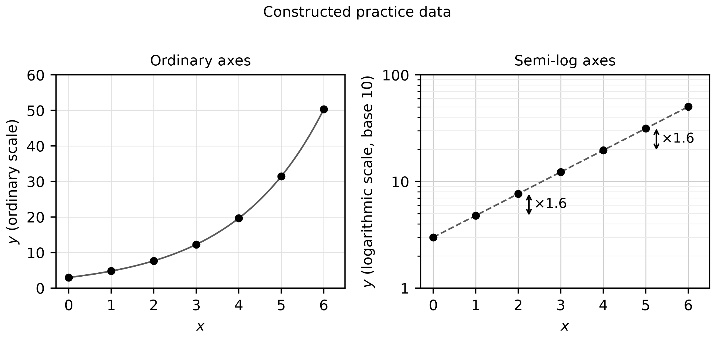
Figure 12.2. The same constructed values of on ordinary axes and on a base-10 logarithmic vertical axis.
Worked example 12.7: from a semi-log line back to an exponential
A semi-log display of constructed data plots against , and its line passes through and . The slope is , so . Exponentiate both sides:
Each unit of multiplies by about 0.779, a decrease of about 22.1%. Check at : the line gives , so , and the model gives as well. The slope does not mean that falls by 0.25 per unit. It is the change in .
Try it 12.3. A line on a semi-log plot of passes through and . Write .
Check your work. The slope is 0.3, so and . Check: .
Worked example 12.8: trust the trend for large inputs
The framework adds a useful point: if the logarithms of the outputs trend linear for large inputs, a transformed exponential such as can model the data, even before you remove the constant . Constructed values of show the idea.
| 0 | 2 | 4 | 6 | 8 | |
|---|---|---|---|---|---|
| 205 | 245 | 605 | 3,845 | 33,005 | |
| 2.312 | 2.389 | 2.782 | 3.585 | 4.519 |
The changes in over each 2 units are 0.077, 0.393, 0.803 and 0.934. They approach , so the plot bends at first and then straightens. A student who demands a constant change across the whole table would reject a model that suits the data.
Error analysis: a check in the wrong place
A student solves , writes , finds or , and confirms both because . The check used the transformed equation, which was built to accept both candidates. The original requires , and is undefined, so the solution is only. The repair is a habit: check in the first line you were given.
Retrieval and review
At your next study session, without notes, write the three-step restriction record and use it to solve the error-analysis equation again on a blank page. About a week later, explain in two sentences why equal vertical gaps on a logarithmic axis mean equal ratios, then convert one semi-log line into an exponential model. In Chapter 20's mixed practice, name the restriction before choosing a method. If a logarithm property caused your error, return to Chapter 11 first.
Practice
Ten multiple-choice questions, Questions 181–190, and one free-response task, Written task 13, are printed after this chapter. Questions 181–186 are no-calculator questions. Questions 187–190 and Written task 13 require a graphing calculator in radian mode. Keys, explanations for every choice and a scoring guide with a complete response are under Chapter 12: answers and explanations. For each miss, record the first incorrect step and the restriction or interpretation you overlooked.