What to practice
- Relate amplitude, midline, period and phase to graphs, tables and an actual context.
Chapter 13 built the sine and cosine graphs from the unit circle. This chapter stretches, shifts and reflects those graphs so that one equation can describe a tide, a turning blade or a daily temperature cycle. It covers topics 3.5 to 3.7 of the AP Precalculus Course and Exam Description. Work in radians throughout, and set your calculator to radian mode before the calculator practice.
Prerequisite check: without looking back, sketch and on and mark where each reaches its maximum. If either sketch is uncertain, review "Build the sine and cosine graphs from the circle" in Chapter 13.
Read the four features of a sinusoid
A sinusoidal function is any function whose graph is a transformation of the sine graph. The cosine graph is itself one: it is the sine graph shifted left by a quarter of a cycle, because for every . Four features describe every sinusoid.
- The period is the length of one full cycle, measured along the input axis. Measure it between matching features: maximum to next maximum, or one rising midline crossing to the next. The frequency is the reciprocal of the period, the number of cycles per unit of input.
- The amplitude is half the vertical distance between a maximum and a minimum: amplitude . It is always positive.
- The midline is the horizontal line halfway between the maximum and minimum values: .
- The phase, or horizontal position, records where a cycle starts relative to the parent graph.
Concavity follows the midline. Between two consecutive midline crossings that surround a maximum, the graph is concave down; around a minimum it is concave up. Each midline crossing is a point of inflection, where the rate of change is greatest in size. Symmetry also carries over: , so sine is an odd function, and , so cosine is even.
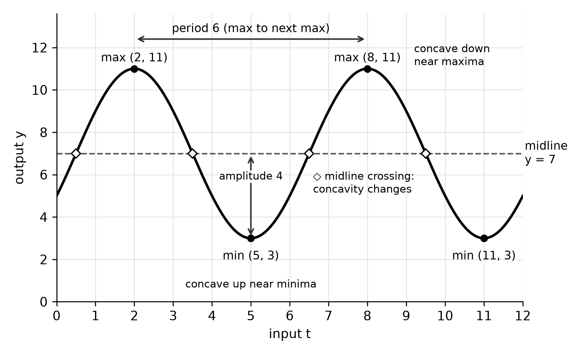
Figure 14.1. One sinusoid with its four features marked. Every measurement in the figure comes from a maximum, a minimum or a midline crossing.
Worked example 14.1: features and behavior from a graph
Read Figure 14.1. The maxima at and give a period of and a frequency of cycle per unit of . The amplitude is and the midline is .
Now describe the function on two quarter-cycles. On the graph falls from a maximum to the midline: it is decreasing and concave down, so its rate of change is negative and decreasing. The graph falls faster and faster. On it is still decreasing but concave up, so the rate of change is negative and increasing toward 0: the graph falls more and more slowly until it reaches the minimum. The same graph can be decreasing on both intervals while its concavity changes, so state direction and concavity separately.
Try it 14.1. A sinusoidal function has a maximum value of 2.6 at , and its next minimum is at . Give the period, frequency, amplitude and midline.
Check your work. A maximum and the next minimum are half a cycle apart, so the period is and the frequency is . The amplitude is and the midline is . Treating 3 as the period is the error to avoid.
Transform sine and cosine with four parameters
Every sinusoid can be written as
with and , and also in the same form with cosine. Each parameter controls one transformation of the parent graph.
| Parameter | Transformation | Feature it sets |
|---|---|---|
| vertical dilation by a factor of ; reflection over the midline when | amplitude | |
| horizontal dilation by a factor of | period | |
| horizontal translation by | phase shift | |
| vertical translation by | midline |
Two habits prevent most errors. First, factor out of the argument before you read the phase shift. In , the graph shifts to the left, not . Second, remember that is not the period: a larger squeezes more cycles into each unit of input, so the period gets shorter.
Worked example 14.2: graph a transformed cosine by quarter-cycles
Graph .
Read the parameters. The amplitude is 3, and reflects the graph, so the cycle begins at a minimum instead of a maximum. The period is . The graph shifts to the right, and the midline is , so the outputs run from to .
Step through quarter-cycles. One quarter of the period is . Start at the shifted input and add four times.
| (minimum) | 1 (midline) | 4 (maximum) | 1 (midline) | (minimum) |
Check one entry by substitution: . Figure 14.2 compares the result with .
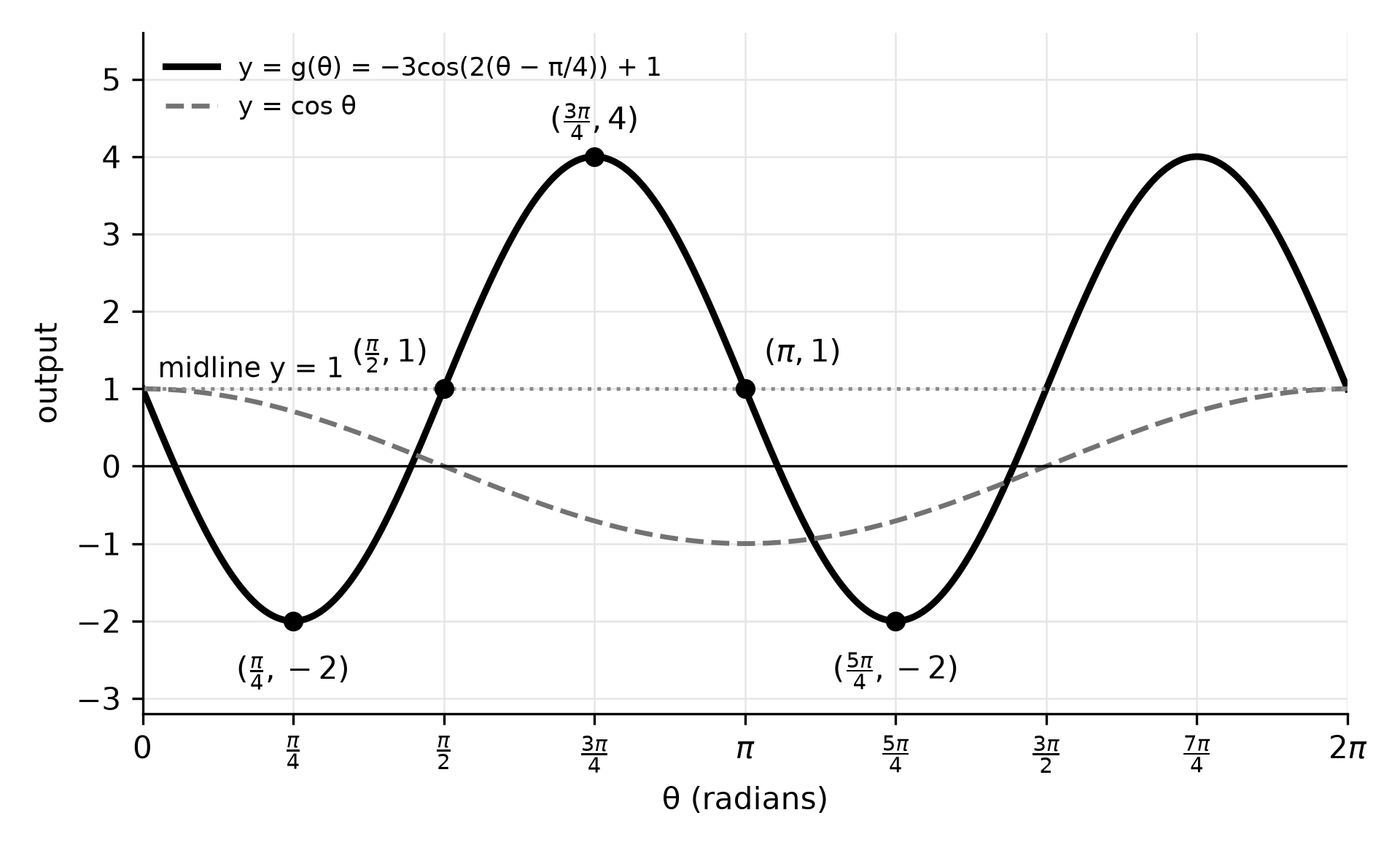
Figure 14.2. The parent cosine (dashed) and its transformation (solid). The reflection moves the start of each cycle to a minimum, and the factor 2 halves the period.
Worked example 14.3: one graph, several equations
An equation for a sinusoid is not unique. For above, the cosine identity gives
All three forms produce the same table. To write an equation from a graph, choose the feature that is easiest to read and match it to a starting shape: starts at a maximum, at a minimum, at a rising midline crossing and at a falling one. For Figure 14.1, the maximum at gives , while the rising midline crossing at gives . Here . Test any candidate with a second labeled point; must give the minimum, 3, in both forms.
Try it 14.2. For , give the amplitude, period, phase shift and range, then find .
Check your work. Factor: . Amplitude 0.5, period , shift to the right, range . Then , a maximum. Reading the shift as is the error to avoid.
Build a model from a context
A context supplies the features directly. Work in this order.
- Name the input and output with units, and decide where is.
- Find the amplitude and midline from the greatest and least outputs.
- Find the period from the context, then .
- Match the starting feature to , , or , and shift if the feature is not at .
- Check the model at a second time from the context, and state the domain on which it applies.
Worked example 14.4: the tip of a turbine blade
The hub of a constructed wind turbine is 30 meters above the ground, each blade is 20 meters long and the rotor turns once every 5 seconds at a steady rate. At seconds, the tip of one blade is at its lowest point. Model the tip's height , in meters.
The highest point is and the lowest is , so the amplitude is 20 and the midline is . The period is 5, so . The motion starts at a minimum, which matches with no shift:
Check: half a turn later, , the top. An equivalent model starts from the rising midline crossing a quarter-turn in: .
Use the model. When is the tip above 40 meters during the first turn? Solve , so . On the argument runs from 0 to , giving or , so or . The tip is above 40 meters for seconds of each turn.
Domain. The model assumes a steady rotation. If the rotor runs at this speed only during a 60-second test, the model's domain is ; it says nothing about the start-up or the slowdown.
Try it 14.3 (partly done). A constructed float on a wave rides highest, 5.2 meters above the sea floor, at seconds and lowest, 3.6 meters, at seconds, and the pattern repeats. The amplitude is 0.8 and the midline is . Finish the model and find the height at .
Check your work. The period is 8, so , and the start at a maximum matches cosine: . At , meters.
Fit a sinusoidal regression to data
When data replace a description, a graphing calculator can fit a sinusoidal regression. Calculators usually report the form . In this form is not the phase shift. Factor out: , so the phase shift is .
Estimate the parameters by hand first, so that you can recognize a fit that has gone wrong. Then interpret the parameters, compute residuals (residual = observed value − predicted value) and keep predictions inside the domain the data support. A positive residual means the model underestimated that observation; a negative residual means it overestimated.
| (hours after midnight) | 0 | 2 | 4 | 6 | 8 | 10 | 12 | 14 | 16 | 18 | 20 | 22 |
|---|---|---|---|---|---|---|---|---|---|---|---|---|
| Temperature (°C) | 16.3 | 14.0 | 14.3 | 16.0 | 18.9 | 22.7 | 25.7 | 27.5 | 28.0 | 26.1 | 22.8 | 18.8 |
The table gives constructed practice data: air temperatures inside a greenhouse, recorded every two hours for one day.
Worked example 14.5: estimate, then regress
Estimate. The greatest reading is 28.0 and the least is 14.0, so the amplitude is about 7 and the midline about 21. The cycle is daily, so the period should be near 24 hours and near . Do not take the period from the two extreme readings. They are 14 hours apart, which would suggest a 28-hour cycle, but readings two hours apart can miss the true low and high.
Regress. Sinusoidal regression in radian mode gives about , , and . The estimates agree. The period is hours and the phase shift is , so the model crosses its midline rising at about 9:05 a.m. Its maximum comes a quarter-period later, near , about 3:00 p.m. A calculator may instead report a negative with changed by , or changed by ; those are the same curve.
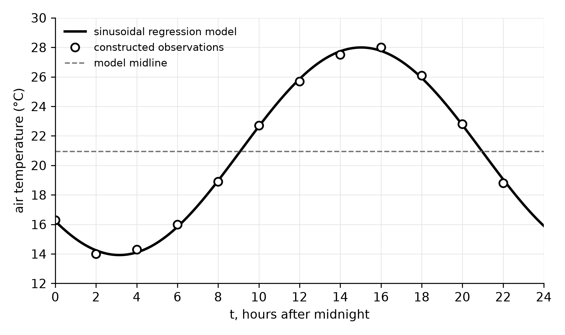
Figure 14.3. Constructed greenhouse temperatures and their sinusoidal regression model. Every observation lies within about 0.26 °C of the curve, and the points fall above and below it in no regular order.
Worked example 14.6: predictions, residuals and limits
Residual. At the model predicts about 27.74 °C. The observed value is 27.5, so the residual is . The model overestimated the temperature at 2:00 p.m. by about 0.24 °C.
Solve with the model. A crop is stressed above 25 °C. Graph the model and and find the intersections: and . The model predicts temperatures above 25 °C from about 11:24 a.m. to 6:39 p.m., roughly 7.3 hours.
Limits. The data cover one day under one set of conditions, so the model's domain is . Its period, 23.8 hours, is close to 24 but not equal to it; over a week the predicted peak would drift by more than an hour, and a cloudy day would change the amplitude. A systematic pattern in the residuals would show that the model is not appropriate, even if every residual were small.
Try it 14.4. A calculator reports the regression . Give the period and the phase shift.
Check your work. The period is . Factor: , so the shift is 2.2 to the right, not 1.1.
Describe behavior quarter by quarter
For with and , each quarter of a cycle has one combination of direction and concavity. Intervals are written as open intervals; including or excluding an endpoint does not change the description.
| Quarter of the cycle | Direction | Concavity | Rate of change |
|---|---|---|---|
| maximum to midline | decreasing | concave down | negative, decreasing |
| midline to minimum | decreasing | concave up | negative, increasing |
| minimum to midline | increasing | concave up | positive, increasing |
| midline to maximum | increasing | concave down | positive, decreasing |
When the cycle starts at a minimum, so read the table from its third row.
Worked example 14.7: behavior in context
For the turbine model, describe the height on . The tip starts at the bottom and reaches the hub level a quarter-turn later, so the interval runs from a minimum to the midline. The height is increasing and the graph is concave up, so the rate of change is positive and increasing: the tip rises faster and faster as it approaches the height of the hub. On it keeps rising, but more and more slowly, until it reaches the top.
Common errors to check
- Period from . The period is , not , and a period read from a maximum to the next minimum must be doubled.
- Unfactored phase shift. In the shift is ; this includes calculator regression output.
- Ignoring the sign of . A negative starts a cosine cycle at a minimum.
- Degree mode. Check one calculator output against the context.
- Residual sign. Residual means observed minus predicted, so a positive residual is an underestimate.
- Extrapolation. A model fitted to one day or one season predicts only within that domain.
Retrieval and review
At your next study session, write the four-parameter form from memory, state which feature each parameter controls, and rebuild the turbine model and the quarter-cycle table without notes. About a week later, rewrite any equation in this chapter in a second form and test both forms at two points. Chapter 15 extends these transformations to tangent.
Practice
Eighteen multiple-choice questions, Questions 205–222, and two free-response tasks, Written tasks 14–15, follow this chapter. Questions 205–214 and both free-response tasks are no-calculator work; Questions 215–222 require a graphing calculator in radian mode. Keys, explanations and scoring rubrics are under Chapter 14: answers and explanations. For each miss, note whether the error came from a feature, a parameter, the phase shift, a residual or the model's domain, then redo the matching worked example before trying a fresh question.