What to practice
- Connect Cartesian and polar views, signed radius, symmetry, graphs and changing distance.
Two ways to name one point
Rectangular coordinates locate a point by horizontal and vertical displacement. Polar coordinates locate the same point by turning and then moving: an angle measured from the positive -axis, called the polar axis, and a signed radial displacement along the line of that angle. The polar grid is a family of circles centered at the origin, or pole, together with lines through it. This chapter converts between the two systems, graphs functions of the form , and describes how a point's distance from the origin changes as increases. One distinction runs through every section: is signed, while the distance from the origin is .
Prerequisite check: give the exact values of and , state the output interval of , and explain what a negative average rate of change means for an ordinary function. Chapter 13 ("Exact values from special triangles") and Chapter 15 ("Restrict and invert") contain the repairs.
Locate a point with an angle and a signed radius
The polar coordinates describe a point in two moves. First draw the terminal ray of in standard position. If , move units from the origin along that ray. If , move units along the same line in the opposite direction. If , the point is the origin, whatever the angle.
The conversion to rectangular coordinates holds for every sign of :
One point has many polar names. Adding to the angle returns to the same ray, so and name the same point for any integer . Adding to the angle while changing the sign of also lands on the same point, so and are equivalent.
Worked example 17.1: a negative radius points backward
Locate the polar point and give its rectangular coordinates.
The terminal ray of points into Quadrant I. Because , move 4 units along the opposite ray, into Quadrant III (Figure 17.1). Then compute.
The point is in Quadrant III, as predicted, and its distance from the origin is . The same point is : add to the angle and change the sign of . Two common errors are plotting in Quadrant I and treating the negative sign as if it made only negative.
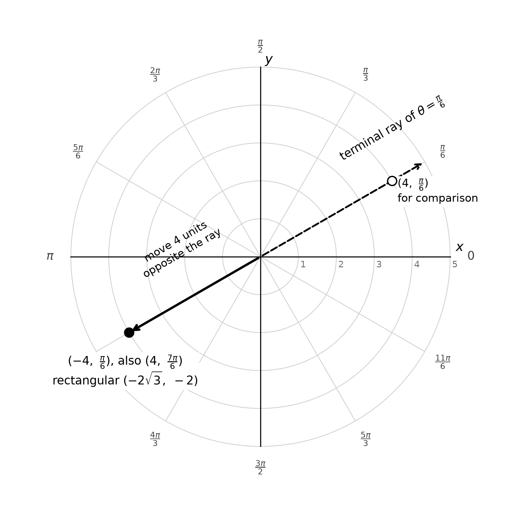
Figure 17.1. A negative radius places the point on the ray opposite the terminal ray of .
Converting from rectangular to polar coordinates
For a point other than the origin, a positive radius is . The angle needs care, because returns values only in , the angles of Quadrants I and IV.
- If , use .
- If , use .
- If , use when and when .
Add or subtract if the question requires an angle in a particular interval, and always convert back as a check.
Worked example 17.2: choose the angle in the correct quadrant
Find polar coordinates of with and .
The radius is . Because , the point is in Quadrant II, but is a Quadrant IV angle. Adding gives . Converting back confirms it: and . The pair also names this point, but it does not meet the stated conditions on and .
Worked example 17.3: a complex number as a point
The complex number corresponds to the point in the complex plane, so it has polar coordinates too. With polar coordinates , the number is .
Write the complex number with polar coordinates in the form , then find polar coordinates of .
First, , a point in Quadrant II as the angle requires. Second, is the point , so ; since , , or in . Check: and .
Graph a polar function from a table
In a polar function , the input is an angle and the output is a signed radius. The graph is the set of points with polar coordinates . Build a table at convenient angles, plot each pair by turning to the angle and then moving the signed distance, and connect the points in order of increasing . A negative output places the point on the opposite side of the origin; it does not disappear from the graph.
Worked example 17.4: trace a limaçon with an inner loop
Graph for .
| 6 | 4 | 2 | 0 | −2 | 0 | 2 | 4 | 6 |
As runs from 0 to , the point moves counterclockwise from through to the origin. From to , is negative, so each point lies opposite its angle. At , gives the rectangular point , on the right of the origin; this piece is the small inner loop. From to , is positive again and the outer curve returns to (Figure 17.2). Check one plotted point by conversion: at , and .
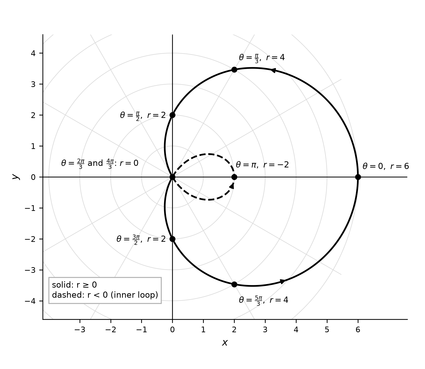
Figure 17.2. The dashed inner loop is traced while the signed radius is negative.
Restricting the input to trace part of a graph
Choosing an input interval selects a portion of a polar graph. For , the inner loop is traced exactly while , which is ; both endpoints place the point at the origin. To find such an interval, solve for the angles at which the desired piece begins and ends, usually where , using the methods of Chapter 16.
Symmetry checked with points
If replacing with leaves unchanged, the graph is symmetric about the polar axis, because is the reflection of across the -axis for either sign of . Since , the graph of has this symmetry, and the table agrees: . Use computed points as evidence rather than the appearance of a sketch.
Describe how distance from the origin changes
For the point , the distance from the origin is . Whether that distance grows depends on both the sign of and its direction of change.
| Signed radius | Distance from the origin |
|---|---|
| positive and increasing | increasing |
| positive and decreasing | decreasing |
| negative and decreasing | increasing |
| negative and increasing | decreasing |
A negative radius that decreases, for example from −1 to −3, carries the point farther from the origin. An increase in does not by itself mean that the point moves away. When crosses 0 inside an interval, split the interval at the crossing and describe each piece separately.
Worked example 17.5: read distance from signed radius
For , describe the distance from the origin on .
Cosine decreases on and increases on , so does the same. The zeros at and split the interval further.
- On , is positive and decreasing, from 2 to 0, so the point approaches the origin.
- On , is negative and decreasing, from 0 to −2, so the point moves away.
- On , is negative and increasing, from −2 to 0, so the point approaches the origin.
- On , is positive and increasing, from 0 to 2, so the point moves away.
Figure 17.3 plots both and against in a rectangular system. The dashed distance graph turns upward wherever the signed radius passes through 0.
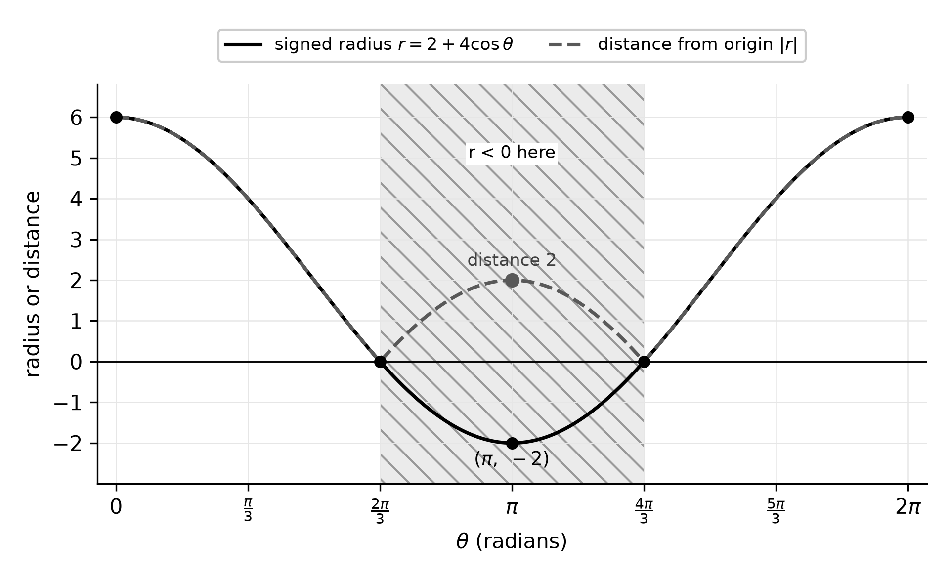
Figure 17.3. Signed radius (solid) and distance from the origin (dashed) for .
Closest and farthest points
Where changes from increasing to decreasing, or from decreasing to increasing, it has a relative extremum, and the corresponding point is relatively closest to or farthest from the origin. Use the sign to decide which. In Worked example 17.5, has a relative minimum of −2 at . Because that radius is negative, the minimum is a point relatively farthest from the origin, at distance 2. Where , at and , the point is the origin itself, the closest possible location.
Average rate of change of the radius
The average rate of change of on is
It measures the change in signed radius per radian, in units of radius per radian. Angles must be in radians; a rate computed with degree measures has a different size and meaning. The average rate can also estimate values inside the interval: if is the average rate on , then , an approximation that is usually better over short intervals.
Worked example 17.6: a rate of signed radius is not a rate of distance
For , find and interpret the average rate of change of on .
Since and , the average rate is , about −2.55 units of radius per radian. The signed radius falls, on average, by about 2.55 units for each radian of rotation. The distance does not: it equals 2 at both endpoints. By Worked example 17.5, the point approaches the origin, reaches it at and then moves away. A negative average rate of change of is not, by itself, a statement that the point got closer.
Worked example 17.7: estimate with a calculator in radian mode
A constructed practice model gives the reach of a lawn sprinkler's spray in direction as meters for . Use the average rate of change on to estimate , then compare with the model's value.
Check the calculator mode first; these angles are radians. Then and , so the average rate is meters per radian. The estimate is meters. The model itself gives meters, so the linear estimate is about 0.17 meter low: the boundary curves outward between the two angles, which a straight-line estimate cannot capture. Here is always positive, so a rate of change of is also a rate of change of distance. In degree mode the calculator would report , a sign that the mode is wrong.
Common errors to check
| Error | Repair |
|---|---|
| Ignoring the sign of when plotting | Worked example 17.1 |
| Using without checking the quadrant | Worked example 17.2 |
| Dropping negative outputs from a polar graph | Worked example 17.4 |
| Treating increasing as moving away from the origin | Worked example 17.5 |
| Reading an average rate of signed radius as a rate of distance | Worked example 17.6 |
| Working in degree mode | Worked example 17.7 |
Try it
Try it 17.1 (partly guided). Give rectangular coordinates for . First predict the quadrant: the ray of points into Quadrant III, so where does a negative radius place the point?
Try it 17.2. Find polar coordinates of with and , then give a second representation with .
Try it 17.3. For , find at and , and say in which quadrant the points for lie.
Try it 17.4. For the same function, is the distance from the origin increasing, decreasing or neither throughout ? Explain.
Check your work.
17.1. The negative radius sends the point into Quadrant I: and , so the point is .
17.2. The point is on the negative -axis, so and . With a negative radius, names the same point: 5 units opposite the ray of .
17.3. The values are . For , is between and , so and each point lies opposite its Quadrant II angle, in Quadrant IV. For example, and give .
17.4. Neither. On this interval decreases from 3 to −3 and crosses 0 at . Before the crossing, is positive and decreasing, so the distance decreases; after it, is negative and decreasing, so the distance increases.
Review and retrieval
Without notes, write the two conversion formulas, the arctangent rule for and the four-row distance table. Tomorrow, replot Figure 17.2 from its table and mark where the signed radius is negative. In about a week, redo Worked example 17.6 and explain in one sentence why the average rate of does not describe distance across a zero. Chapter 18 develops the calculator workflow behind the last six practice questions, and Chapter 20 mixes these skills with earlier units.
Practice
Eighteen multiple-choice questions (Questions 251–268) are printed after this chapter under Printed practice. Questions 251–262 are for work without a calculator. Questions 263–268 require a graphing calculator in radian mode, and each says so in its first sentence. The keys and the reasoning behind every choice are under Chapter 17: answers and explanations. For each miss, decide whether the error involved the sign of , the quadrant of an angle, distance versus signed radius, or the calculator mode, and redo the matching worked example before a fresh attempt.