What to practice
- Introduce the untested unit with connected examples and clear limits of coverage.
Read this first: an optional chapter
This chapter is optional. It introduces Unit 4 of the AP Precalculus course framework: functions involving parameters, vectors and matrices. Teachers may include Unit 4 to meet state or local requirements, but the AP Precalculus Course and Exam Description states that it is not assessed on the AP exam. Nothing here appears in this book's practice exams or numbered questions, and skipping the chapter does not weaken your exam preparation.
Read it if your class covers Unit 4, if you plan to take AP Calculus BC, physics or linear algebra, or if you want to see where the rate-of-change ideas of Chapter 3 lead. Every main heading is marked optional. Try-it tasks with full solutions follow the demonstrations.
Parametric functions describe motion (optional)
A parametric function gives both coordinates of a point in terms of a third variable, the parameter, usually : the point is . Think of as time. Each value of places the point somewhere in the plane, and as increases the point traces a path. The stated interval of fixes a starting point and an ending point. When is increasing the point moves right, and when is increasing it moves up.
Worked demonstration 21.1: table, path and direction
Let and for .
| 0 | 1 | 2 | 3 | ||
|---|---|---|---|---|---|
| 3 | 0 | 0 | 3 | ||
| 1 | 3 | 5 |
The path starts at when and ends at when (Figure 21.1). Because always increases, the point always moves up. Because decreases for and increases for , it moves left and then right, so its leftmost point is at . It crosses the -axis when , at , where . It crosses the -axis when , at and .
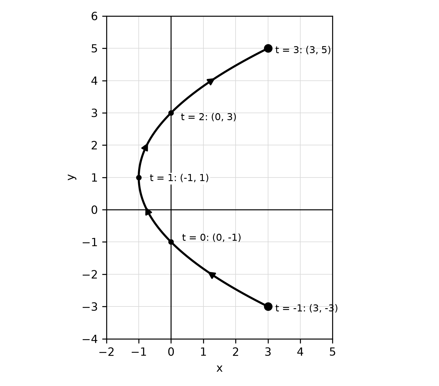
Figure 21.1. A parametric path with its direction of motion.
The path is not the graph of a function of , because matches two points. It is, however, a function of . Since , substituting gives .
Worked demonstration 21.2: rates along a path
The average rate of change of over is , and likewise for . When changes, the slope of the segment joining the two points on the path is the ratio of these rates, .
Over , and . Each coordinate changes at an average of 2 units per unit of , and the segment has slope . Over , and , so the slope is . Over , : the segment from to is vertical and has no slope, even though the point kept moving.
Worked demonstration 21.3: circles and segments
The point for travels once around the unit circle, counterclockwise from . Scaling and shifting gives any circle: center and radius come from and . For center and radius 3, use and , which starts at . Replacing by reverses the direction to clockwise.
A segment uses linear coordinate functions. From to , try and for . At the point is , and at it is . Both coordinates change at constant rates, 2 and , so the path is straight with slope .
Any function can be written as , and its inverse relation as .
Implicit relations and conic sections (optional)
An equation in and can define a curve without solving for either variable. Such a relation is defined implicitly. The circle is an example: it contains both and , so it is not the graph of a function of .
Worked demonstration 21.4: a circle as two functions
Solving for gives two functions on : the upper half and the lower half (Figure 21.2, panel A). Together they make up the relation. Chapter 3's tools apply to each piece. On the upper half, the average rate of change over is , and over it is . The curve falls faster near the edge.
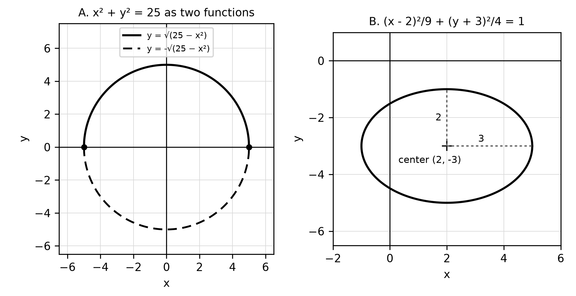
Figure 21.2. (a) An implicit relation split into two functions. (b) An ellipse in standard form.
Worked demonstration 21.5: complete the square to name a conic
The three conic sections have standard forms. A parabola can be written or . An ellipse centered at is . A hyperbola is , opening left and right, or , opening up and down.
Identify . Group and factor: . Complete each square: , so . Dividing by 36,
This is an ellipse centered at with horizontal radius 3 and vertical radius 2 (Figure 21.2, panel B). A parametrization is , for . Check one point: gives , and .
Worked demonstration 21.6: a hyperbola and its asymptotes
For , the center is , and . The hyperbola opens left and right through the vertices , and its asymptotes are . In general, the asymptotes are . At the curve has , so , while the asymptotes give . The curve stays between them. Because , the right branch is parametrized by , for .
Vectors: magnitude and direction (optional)
A vector has magnitude and direction. Draw it as an arrow from a tail to a head. The vector from to has components . For :
- its magnitude is ;
- the scalar multiple is times as long and points the opposite way when ;
- sums add components, , which places the arrows head to tail;
- a unit vector in the direction of is , and and let you write ;
- a vector of magnitude at direction angle is ;
- the dot product is , which equals for the angle between them, so two nonzero vectors are perpendicular exactly when their dot product is 0.
Worked demonstration 21.7: components, unit vectors and the dot product
From to , . Its magnitude is , and the unit vector in its direction is , or . Adding gives . Next, , so those two vectors are perpendicular. A vector of magnitude 12 at is , about .
Worked demonstration 21.8: two forces, two methods
Forces of 5 newtons and 8 newtons pull on one point, with between them. Find the magnitude of their sum.
Components. Put the first force along the -axis: , with magnitude newtons.
Law of cosines. In the parallelogram the forces form, the sum is the diagonal opposite an angle of . So , and newtons again.
Worked demonstration 21.9: a position vector that moves
A vector-valued function gives a position vector for each . Rewrite Demonstration 21.1 as . The magnitude is the distance from the origin at . The displacement from to is , so the average velocity is units per unit of . Its magnitude, , is a straight-line distance per unit of ; the curved path between the two points is longer. Velocity at an instant, and speed as its magnitude, come from the same average rates over shrinking intervals.
Matrices act on vectors (optional)
A matrix is a rectangular array of numbers; this section uses matrices. Multiply two matrices row by column: the entry in row and column of is the dot product of row of with column of . The identity matrix, with 1s on the diagonal and 0s elsewhere, leaves every vector unchanged. For
the determinant is . The inverse exists exactly when , and then . The value is the area of the parallelogram formed by the two column vectors, and exactly when they are parallel.
Worked demonstration 21.10: order matters
For instance, row 1 of times column 2 of is , while row 1 of times column 2 of is . So . Apply each product to the vector . applies first: sends to , and sends that to . applies first, giving and then .
Worked demonstration 21.11: determinant, inverse and a system
Let have rows and . Then , so
Multiplying by gives the identity. The system , is applied to equal to , so . Check: and . Its columns, and , span a parallelogram of area . By contrast, the matrix with rows and has determinant . Its columns and are parallel, and it has no inverse.
Worked demonstration 21.12: a transformation built from unit vectors
A linear transformation has the form . Its matrix is found from where it sends and : those images are the columns. Suppose . Then and , so
The unit square maps to the parallelogram with vertices , , and (Figure 21.3). Its area is , and every region's area is doubled. The inverse transformation uses , which sends back to . A counterclockwise rotation by has columns and ; for it sends to . Doing one transformation and then another corresponds to multiplying their matrices, with the first one on the right.
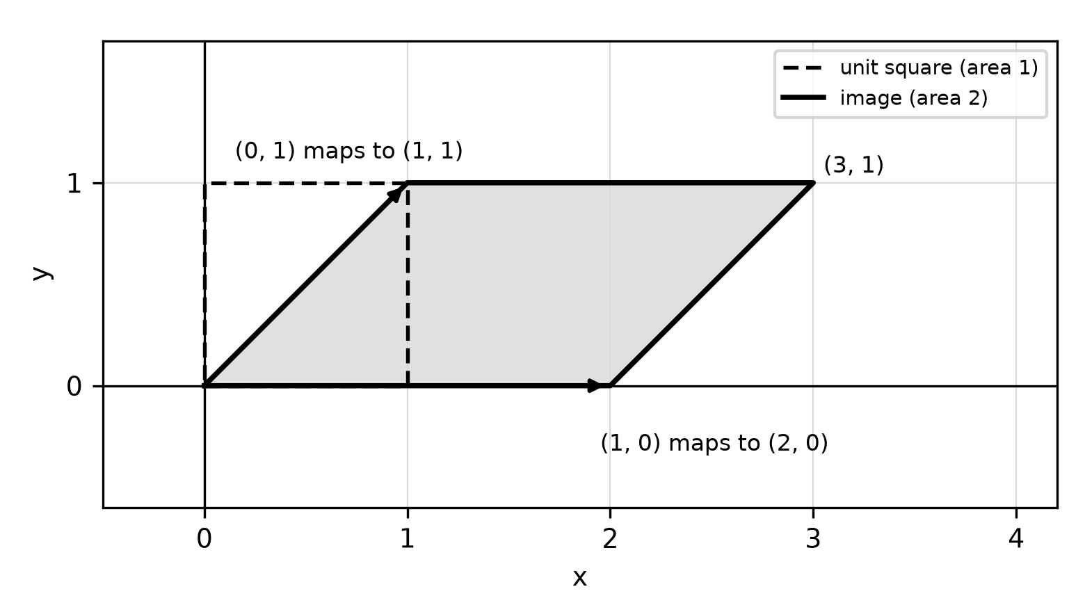
Figure 21.3. A linear transformation and its area factor, the determinant.
Worked demonstration 21.13: a transition model
Two bike-share stations, North and South, exchange bicycles every hour (constructed practice data). Each hour, 80% of the bikes at North stay and 20% move to South; 70% at South stay and 30% move to North. With the state vector , the transition matrix has columns "from North" and "from South":
Start with . One hour later the state is , and after two hours it is . A steady state satisfies . Then , so and ; with 1,000 bikes this is . To look one hour into the past, use the inverse. Since ,
and . Check: .
Try it (optional)
Parameters.
- For and with , give the starting and ending points, describe the horizontal and vertical motion, and find the slope of the segment between the points at and .
- Parametrize the circle with center and radius 4, traced counterclockwise from .
Conics.
- Write in vertex form and give a parametrization.
- Give the center and asymptotes of .
Vectors.
- For and , find , the unit vector in the direction of , and the value of that makes and perpendicular.
- For , find the displacement and the average velocity from to .
Matrices.
- For the matrix with rows and , find and . Are its columns parallel?
- Using from Demonstration 21.13, find the state three hours after .
Check your try-it work (optional)
- Start , end . The point moves left because decreases, and up because increases. The points are and , so the slope is .
- , for . At the point is .
- , so : a parabola opening right with vertex . One parametrization is , .
- Center , , , opening up and down. The asymptotes are .
- ; the unit vector is . Perpendicular requires , so .
- and . The displacement is and the average velocity is .
- , so has rows and . The determinant is not 0, so the columns are not parallel.
- From : . The states approach the steady state .
Where to go next (optional)
The circle parametrization relies on the unit circle of Chapter 13, and Chapter 17's polar paths also trace a point as a parameter changes. Rates along a path extend Chapter 3's average rates and return in calculus; matrices and transformations begin linear algebra.
Practice (optional)
This chapter has no numbered questions, and no practice exam item depends on it. Its practice is the thirteen worked demonstrations and the eight try-it tasks above, with complete solutions under Check your try-it work.